Panel Data Modeling in R
Introduction
This presentation demonstrates panel data modeling using the plm package in R. We will use the Produc dataset, which contains data on gross state product in the United States.
Load Libraries and Data
Data Description
The Produc dataset contains the following variables:
-
state: State name -
year: Year -
region: Region -
pcap: Real per capita personal consumption expenditures -
hwy: Real per capita “highway” expenditure -
water: Real per capita “water” expenditure -
util: Real per capita “utility” expenditure -
pc: Real per capita net income -
gsp: Real gross state product -
emp: Employment -
unemp: Unemployment rate
Ploting GSP over Time
ggplot(Produc, aes(x = year, y = gsp, color = state)) +
  geom_line() +
  theme_minimal() +
  labs(title = "Gross State Product over Time",
       x = "Year",
       y = "Gross State Product (GSP)")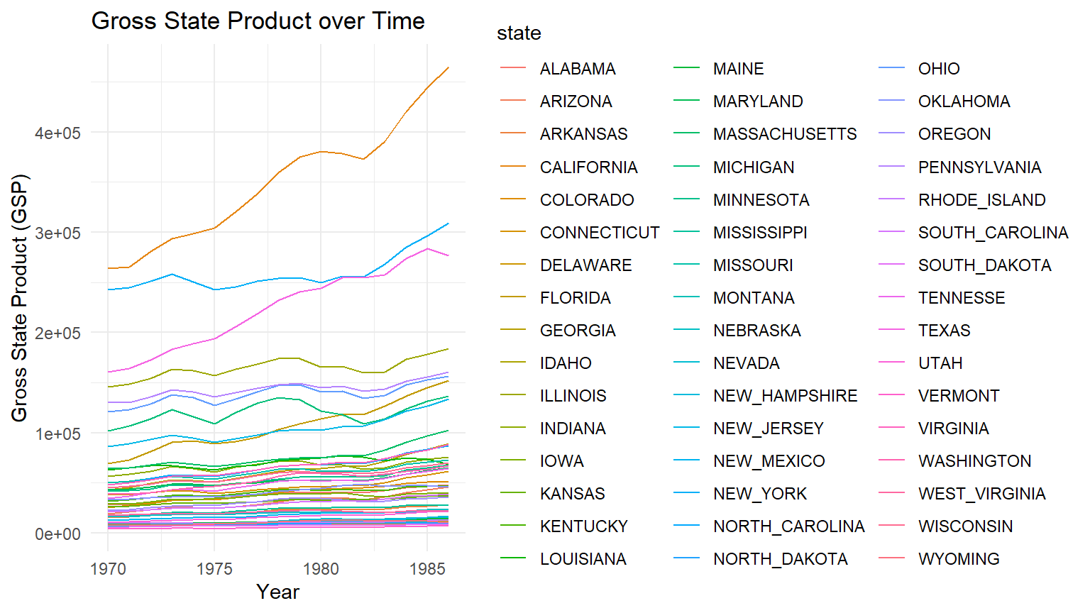
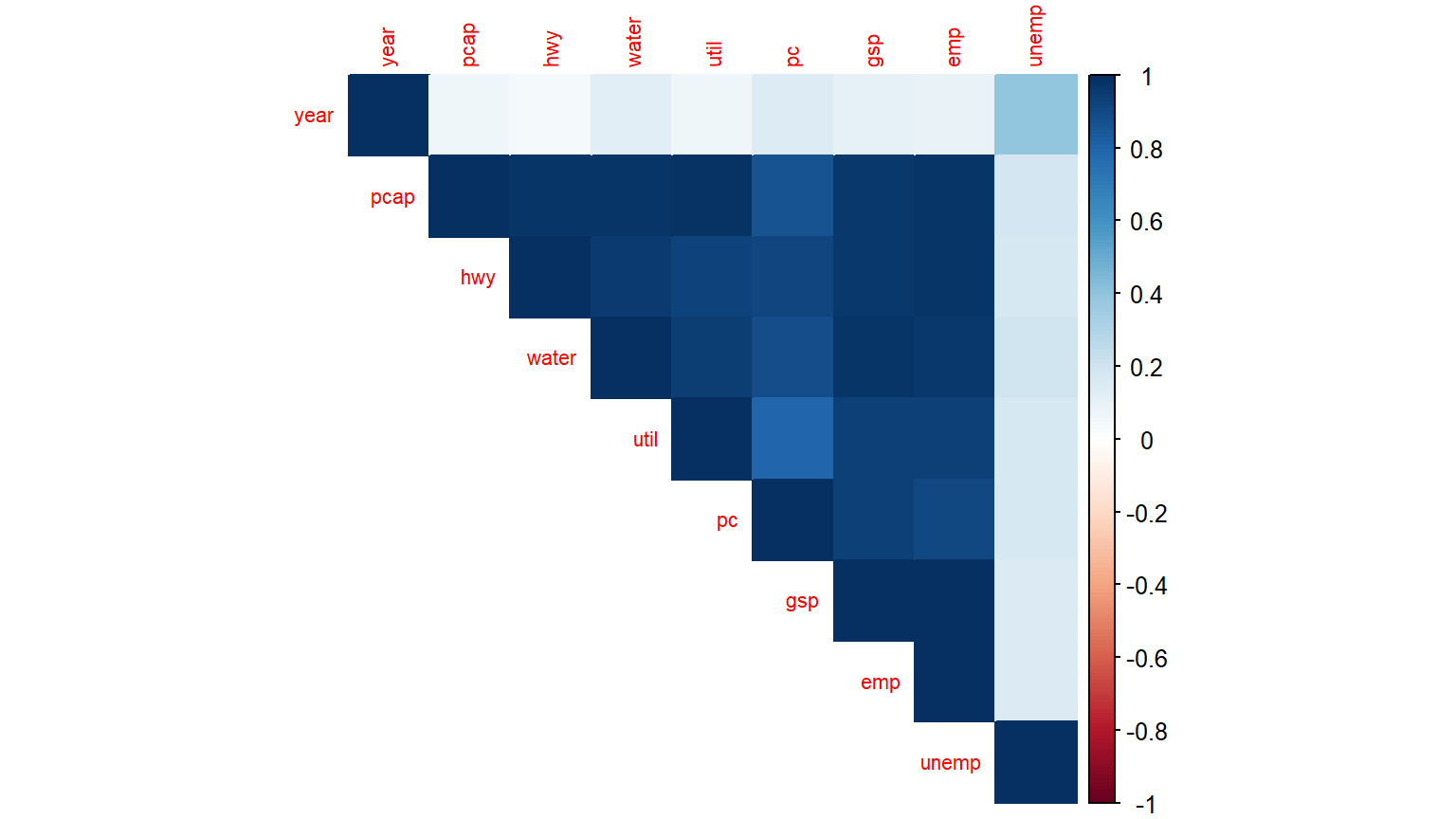
Correlation plot
Boxplot of GSP by Region
ggplot(Produc, aes(x = region, y = gsp, fill = region)) +
  geom_boxplot() +
  theme_minimal() +
  labs(title = "Gross State Product by Region",
       x = "Region",
       y = "Gross State Product (GSP)")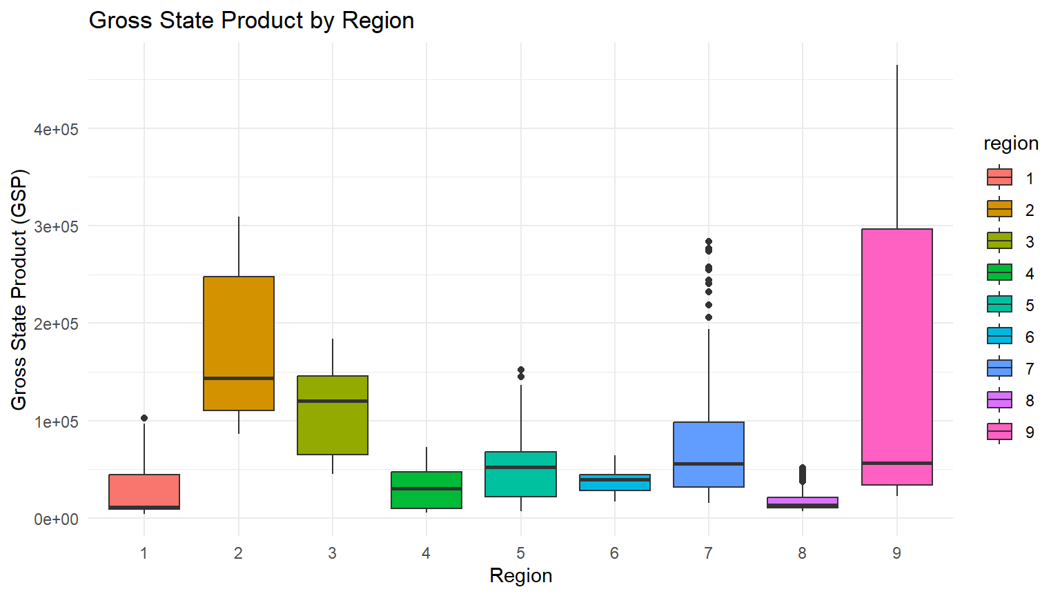
Boxplot of Employment by Region
ggplot(Produc, aes(x = region, y = emp, fill = region)) +
  geom_boxplot() +
  theme_minimal() +
  labs(title = "Employment by Region",
       x = "Region",
       y = "Employment")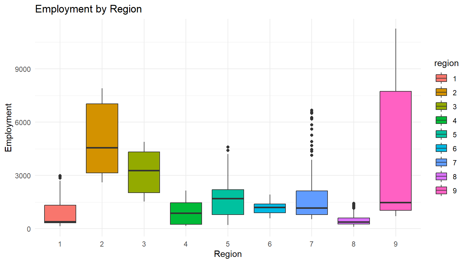
Scatterplot of GSP vs. Employment by State
ggplot(Produc, aes(x = emp, y = gsp, color = state)) +
  geom_point() +
  theme_minimal() +
  labs(title = "Gross State Product vs. Employment by State",
       x = "Employment",
       y = "Gross State Product (GSP)")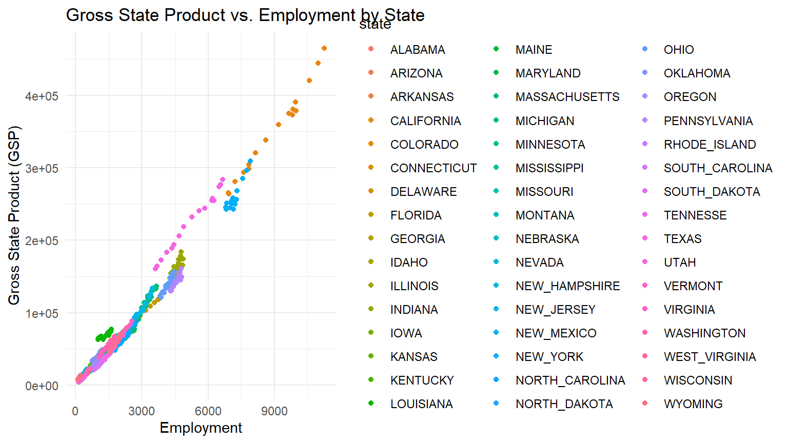
Unit Root Tests
 pcap   hwy water  util    pc   gsp   emp unemp
 0.01  0.01  0.01  0.01  0.01  0.01  0.01  0.01
Fit Pooled OLS Model
Pooled OLS model
Pooling Model

Call:
plm(formula = gsp ~ emp + unemp + pc, data = Produc, model = "pooling")

Balanced Panel: n = 48, T = 17, N = 816

Residuals:
   Min. 1st Qu.  Median 3rd Qu.    Max.
 -26662   -4069    1503    3784   40850

Coefficients:
               Estimate  Std. Error t-value  Pr(>|t|)
(Intercept) -3.8305e+03  8.0097e+02 -4.7824 2.057e-06 ***
emp          3.0144e+01  3.2554e-01 92.5964 < 2.2e-16 ***
unemp       -3.4768e+02  1.1538e+02 -3.0133  0.002665 **
pc           2.4878e-01  1.0142e-02 24.5292 < 2.2e-16 ***
---
Signif. codes:  0 '***' 0.001 '**' 0.01 '*' 0.05 '.' 0.1 ' ' 1

Total Sum of Squares:    3.9905e+12
Residual Sum of Squares: 4.2567e+10
R-Squared:      0.98933
Adj. R-Squared: 0.98929
F-statistic: 25103.7 on 3 and 812 DF, p-value: < 2.22e-16
Fixed Effects Model
Oneway (individual) effect Within Model

Call:
plm(formula = gsp ~ emp + unemp + pc, data = Produc, model = "within")

Balanced Panel: n = 48, T = 17, N = 816

Residuals:
    Min.  1st Qu.   Median  3rd Qu.     Max.
-12824.8   -912.6    -50.2    720.4  20701.7

Coefficients:
         Estimate  Std. Error t-value  Pr(>|t|)
emp     34.611677    0.926593 37.3537 < 2.2e-16 ***
unemp -289.266470   59.882397 -4.8306 1.645e-06 ***
pc       0.134576    0.021505  6.2579 6.495e-10 ***
---
Signif. codes:  0 '***' 0.001 '**' 0.01 '*' 0.05 '.' 0.1 ' ' 1

Total Sum of Squares:    1.3289e+11
Residual Sum of Squares: 5628300000
R-Squared:      0.95765
Adj. R-Squared: 0.95488
F-statistic: 5765.77 on 3 and 765 DF, p-value: < 2.22e-16
Random Effects Model
Oneway (individual) effect Random Effect Model
   (Swamy-Arora's transformation)

Call:
plm(formula = gsp ~ emp + unemp + pc, data = Produc, model = "random")

Balanced Panel: n = 48, T = 17, N = 816

Effects:
                   var  std.dev share
idiosyncratic  7357308     2712 0.132
individual    48523782     6966 0.868
theta: 0.906

Residuals:
   Min. 1st Qu.  Median 3rd Qu.    Max.
 -12212    -893     153     873   20740

Coefficients:
               Estimate  Std. Error z-value  Pr(>|z|)
(Intercept) -4347.08517  1193.82256 -3.6413 0.0002712 ***
emp            33.06917     0.73227 45.1600 < 2.2e-16 ***
unemp        -331.96706    57.93287 -5.7302 1.003e-08 ***
pc              0.16804     0.01800  9.3353 < 2.2e-16 ***
---
Signif. codes:  0 '***' 0.001 '**' 0.01 '*' 0.05 '.' 0.1 ' ' 1

Total Sum of Squares:    1.6699e+11
Residual Sum of Squares: 6012600000
R-Squared:      0.96399
Adj. R-Squared: 0.96386
Chisq: 21740.2 on 3 DF, p-value: < 2.22e-16
Hausman Test
hausman_test <- phtest(fixed_effects, random_effects)
hausman_test
    Hausman Test

data:  gsp ~ emp + unemp + pc
chisq = 7.9388, df = 3, p-value = 0.04729
alternative hypothesis: one model is inconsistent
Model comparison Breusch-Pagan test
bp_test <- plmtest(fixed_effects, effect = "twoways", type = "bp")
bp_test
    Lagrange Multiplier Test - two-ways effects (Breusch-Pagan)

data:  gsp ~ emp + unemp + pc
chisq = 4755.8, df = 2, p-value < 2.2e-16
alternative hypothesis: significant effects
Model comparison F-test
f_test <- pFtest(fixed_effects, random_effects)
f_test
    F test for individual effects

data:  gsp ~ emp + unemp + pc
F = 1.1113, df1 = 47, df2 = 765, p-value = 0.2856
alternative hypothesis: significant effects
Robustness Check with Clustered Standard Errors
t test of coefficients:

         Estimate  Std. Error t value Pr(>|t|)
emp     34.611677    2.731771 12.6701  < 2e-16 ***
unemp -289.266470  123.251462 -2.3470  0.01918 *
pc       0.134576    0.069376  1.9398  0.05277 .
---
Signif. codes:  0 '***' 0.001 '**' 0.01 '*' 0.05 '.' 0.1 ' ' 1
Summary
This presentation demonstrated panel data modeling using the plm package in R. We covered data exploration, unit root testing, fitting pooled, fixed, and random effects models, and comparing these models using statistical tests.
These results can help us understand the relationships between gross state product and other economic indicators while accounting for individual state effects.
From this analysis, we can conclude that the fixed effects model is preferred over the random effects model based on the Hausman test results. The pooled OLS model is not appropriate due to the presence of individual-specific effects.