Spurious Regression

Zahid Asghar

Complete Blog on Spurious Regression

https://zahidasghar.com/timeseries/spurious_regression

Spurious Regression

\(y_t = a_0 + a_1z_t + e_t\)

where \(y_t\) is the dependent variable, \(z_t\) is the independent variable, \(a_0\) and \(a_1\) are the parameters, and \(e_t\) is the error term. Assumptions of the classical model:

• both the {\(y_t\)} and {\(z_t\)} sequences be stationary

• the errors have a zero mean and a finite variance.

In the presence of nonstationary variables, there might be what Granger and Newbold (1974) call a spurious regression.

A spurious regression has a high \(R^2\) and \(t\)-statistics that appear to be significant, but the results are without any economic meaning. The regression output “looks good” because the least-squares estimates are not consistent and the customary tests of statistical inference do not hold.

CASE 1: Both {yt} and {zt} are stationary. The classical regression model is appropriate.

CASE 2: The {yt} and {zt} sequences are integrated of different orders. Regression equations using such variables are meaningless.

CASE 3: The nonstationary {yt} and {zt} sequences are integrated of the same order and the residual sequence contains a stochastic trend. This is the case in which the regression is spurious. In this case, it is often recommended that the regression equation be estimated in first differences.

CASE 4: The nonstationary {yt} and {zt} sequences are integrated of the same order and the residual sequence is stationary. In this circumstance, {yt} and {zt} are cointegrated.

Load libraries and generate data

library(tidyverse) # An umbrella package that installs the tidyverse packages

library(readxl) # To read excel files

library(broom) # To tidy up the regression output

library(moderndive) # To get regression points

library(ggfortify) # To plot regression diagnostics

library(ggResidpanel) # To plot regression diagnostics

Simulate data

T <- 200
set.seed(1357)
y <- ts(rep(0,T))
vy <- ts(rnorm(T))
for (t in 2:T){
  y[t] <- y[t-1]+vy[t]
}

set.seed(4365)
x <- ts(rep(0,T))
vx <- ts(rnorm(T))
for (t in 2:T){
  x[t] <- x[t-1]+vx[t]
}
y <- ts(y[50:200])
x <- ts(x[50:200])

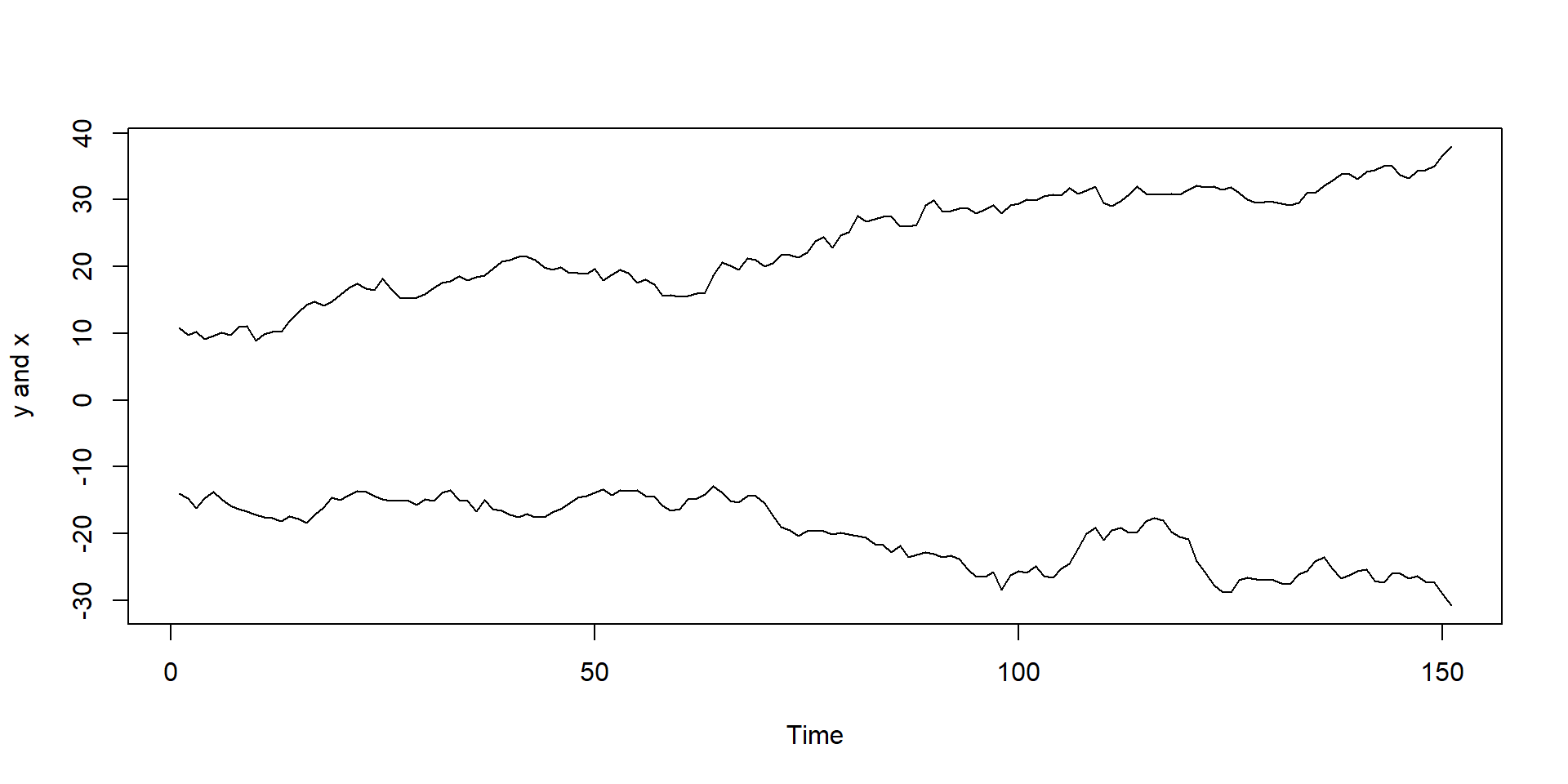
Plot the data

ts.plot(y,x, ylab="y and x")

summary(lm(y~x))

Call:
lm(formula = y ~ x)

Residuals:
    Min      1Q  Median      3Q     Max 
-6.1121 -2.0348  0.1727  2.0074  6.1537 

Coefficients:
            Estimate Std. Error t value Pr(>|t|)    
(Intercept)  -7.1351     0.7252  -9.839   <2e-16 ***
x            -0.5410     0.0293 -18.464   <2e-16 ***
---
Signif. codes:  0 '***' 0.001 '**' 0.01 '*' 0.05 '.' 0.1 ' ' 1

Residual standard error: 2.737 on 149 degrees of freedom
Multiple R-squared:  0.6959,    Adjusted R-squared:  0.6938 
F-statistic: 340.9 on 1 and 149 DF,  p-value: < 2.2e-16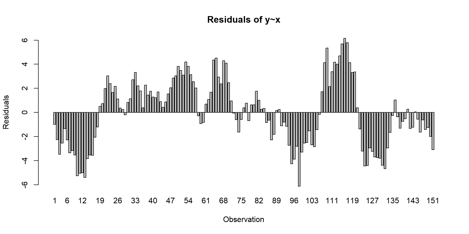

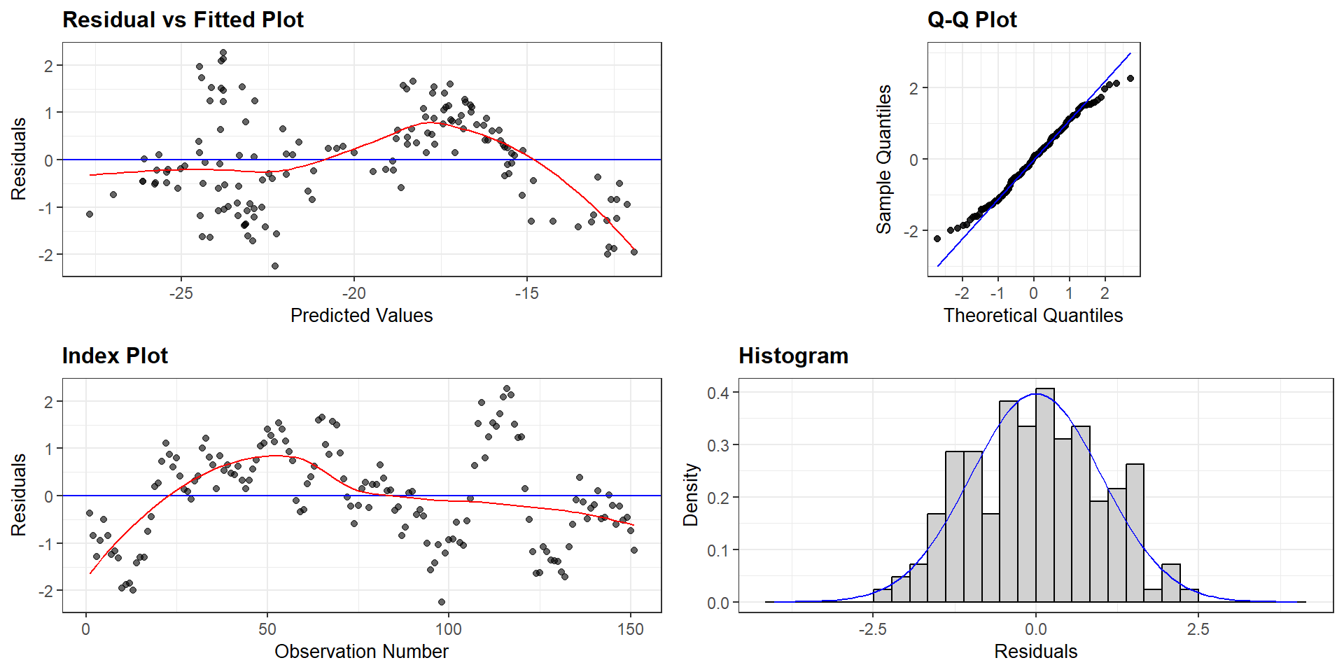
# barplot of residuals
resid <- residuals(lm(y~x))
barplot(resid, ylab="Residuals", xlab="Observation", main="Residuals of y~x")

Residuals panel

resid_panel(lm(y~x))