Main Objectives
Concept of cointegration
Studying the dynamics of cointegrated variables
Methods for testing cointegration
How to estimate a system of cointegrated variables
VAR and VECM difference
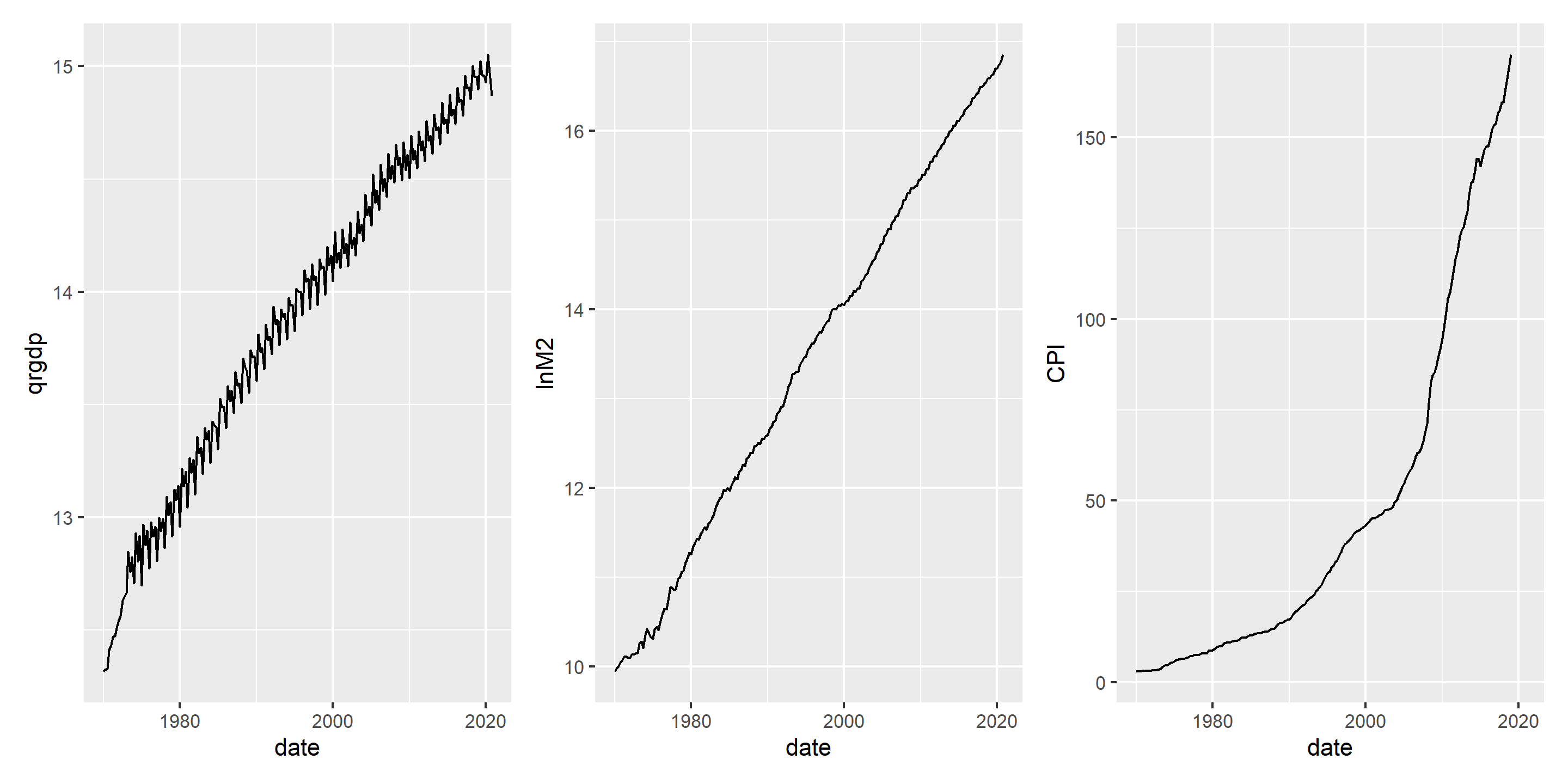
Graphs of data
## # A tibble: 204 × 12
##    date...1            quarter Quarter  Year date...5  QRGDP M2_mill_rs
##    <dttm>                <dbl> <chr>   <dbl> <chr>     <dbl>      <dbl>
##  1 1970-01-01 00:00:00       1 Q1       1970 1970Q1   223168      20800
##  2 1970-04-01 00:00:00       2 Q2       1970 1970Q2   225140      21500
##  3 1970-07-01 00:00:00       3 Q3       1970 1970Q3   225980      22213
##  4 1970-10-01 00:00:00       4 Q4       1970 1970Q4   245436      22965
##  5 1971-01-01 00:00:00       1 Q1       1971 1971Q1   251348      23632
##  6 1971-04-01 00:00:00       2 Q2       1971 1971Q2   259999      24643
##  7 1971-07-01 00:00:00       3 Q3       1971 1971Q3   261355      24718
##  8 1971-10-01 00:00:00       4 Q4       1971 1971Q4   271232      24300
##  9 1972-01-01 00:00:00       1 Q1       1972 1972Q1   279965      24324
## 10 1972-04-01 00:00:00       2 Q2       1972 1972Q2   285432      25134
## # ℹ 194 more rows
## # ℹ 5 more variables: LNRGDP <dbl>, LNM2 <dbl>, CPI <dbl>, inf <dbl>,
## #   `inf cpi` <dbl>
![]()
These graphs indicate all three variables are non-stationary.
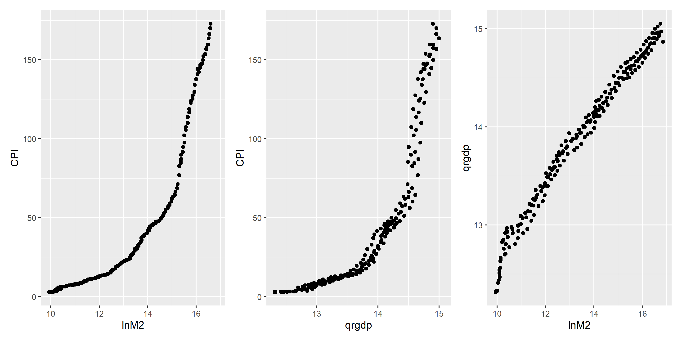
Scatter plot of the variables
![]()
Money and Price
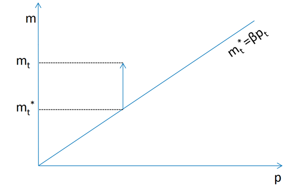
Suppose that in the long run \(m_t=\beta p_t+e_t\) where \(\beta>0\) That is \(m_t\) and \(p_t\) are cointegrated and money nuetrality hypothesis would imply \(\beta=1\). If \(m \uparrow\) s.t \(m_t-\beta p_t>0\), what would be the dynamics?
Deviation and now what
![]()
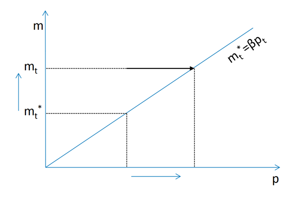
\(m_t\) is doing all the adjument
![]()
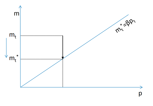
\(m^*_t\) is unchanged and \(m_t\) \(\downarrow\)
\(\Delta m_t=\alpha_m(m_{t-1}-m^*_{t-1})\) where \(\alpha_m<0\) Short run change in \(m_t\) is a linear function of the deviation from the long run from the long run equilibrium
\(m^*_t\) is doing all the adjument
![]() \(m_t\) is unchanged and \(p_t\) and \(m^*_t\) \(\uparrow\) \(\Delta p_t=\alpha_p(m_{t-1}-m^*_{t-1})\) where \(\alpha_p>0\) Short run change in \(p_t\) is a linear function of the deviation from the long run from the long run equilibrium
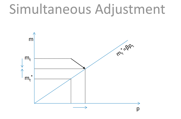
Both \(m_t\) and \(p_t\) adjust
![]() \(m_t\) and \(p_t\) are adjusting simultaneously \(\Delta m_t=\alpha_m(m_{t-1}-m^*_{t-1})\) \(\Delta p_t=\alpha_p(m_{t-1}-m^*_{t-1})\) which is basically error/equilibrium correction model. !…
Both \(m_t\) and \(p_t\) adjust simulataneously
![]()
\(m_t\) and \(p_t\) are adjusting simultaneously \(\Delta m_t=\alpha_m(m_{t-1}-m^*_{t-1})\) \(\Delta p_t=\alpha_p(m_{t-1}-m^*_{t-1})\)
Cointegration and VECM (Continued)
Simple ECM \(m_t\) and \(p_t\) are cointegrated with adjustment in \(e_t\) \(\Delta m_t=\alpha_m(m_{t-1}-\beta p_{t-1})+\nu_t\) \(\Delta p_t=\alpha_p(m_{t-1}-\beta p_{t-1})+\mu_t\) A VAR in difference would be misspecified.
\(m_t=(1+\alpha_m)m_{t-1}-\alpha_m \beta p_{t-1}+\nu_t\)
\(p_t=\alpha_p m_{t-1}-(1-\alpha_p \beta) p_{t-1}+\mu_t\)
These two equations represent VAR but with nonlinear constraints on its coefficients.
Back to money, prices and gdp issue
Economic theory indicate that \(m_t\), \(p_t\) and \(y_t\) are cointegrated. Lets write simple VECM of order zero
No lags of \(\Delta m_t\),\(\Delta p_t\) and \(\Delta y_t\) \(\Delta m_t=\alpha_m(\beta_1 m_{t-1}+\beta_2 p_{t-1}+\beta_3 y_{t-1}+\beta_4)+\nu_t\)
\(\Delta p_t=\alpha_p(\beta_1 m_{t-1}+\beta_2 p_{t-1}+\beta_3 y_{t-1}+\beta_4)+\mu_t\)
\(\Delta y_t=\alpha_y(\beta_1 m_{t-1}+\beta_2 p_{t-1}+\beta_3 y_{t-1}+\beta_4)+\eta_t\)
VECM of order 1
\(\Delta m_t=\alpha_m(\beta_1 m_{t-1}+\beta_2 p_{t-1}+\beta_3 y_{t-1}+\beta_4)+\\ \lambda_{mm} \Delta m_{t-1}+\lambda_{mp} \Delta p_{t-1}+\lambda_{my} \Delta y_{t-1}+\nu_t\)
\(\Delta p_t=\alpha_p(\beta_1 m_{t-1}+\beta_2 p_{t-1}+\beta_3 y_{t-1}+\beta_4)+\\ \lambda_{pm} \Delta m_{t-1}+\lambda_{pp} \Delta p_{t-1}+\lambda_{py} \Delta y_{t-1}\mu_t\)
\(\Delta y_t=\alpha_y(\beta_1 m_{t-1}+\beta_2 p_{t-1}+\beta_3 y_{t-1}+\beta_4)+\\ \lambda_{ym} \Delta m_{t-1}+\lambda_{yp} \Delta p_{t-1}+\lambda_{yy} \Delta y_{t-1}+\eta_t\)
Deterministic component
Case 1 \(\Delta m_t=\alpha_m(\beta_1 m_{t-1}+\beta_2 p_{t-1}+\beta_3 y_{t-1}+\beta_4)+\\\lambda_{mm} \Delta m_{t-1}+\lambda_{mp} \Delta p_{t-1}+\lambda_{my} \Delta y_{t-1}+\nu_t\)
Case 2
\(\Delta m_t=\alpha_m(\beta_1 m_{t-1}+\beta_2 p_{t-1}+\beta_3 y_{t-1}+\beta_4)+\\\lambda_{mm} \Delta m_{t-1}+\lambda_{mp} \Delta p_{t-1}+\lambda_{my} \Delta y_{t-1}+\nu_t\)
Case 3
\(\Delta m_t=\mu_m+\alpha_m(\beta_1 m_{t-1}+\beta_2 p_{t-1}+\beta_3 y_{t-1}+\beta_4)+\\\lambda_{mm} \Delta m_{t-1}+\lambda_{mp} \Delta p_{t-1}+\lambda_{my} \Delta y_{t-1}+\nu_t\)
Case 3 VECM order 1 with constant
\(\Delta m_t=\mu_m+\alpha_m(\beta_1 m_{t-1}+\beta_2 p_{t-1}+\beta_3 y_{t-1}+\beta_4)+\\\lambda_{mm} \Delta m_{t-1}+\lambda_{mp} \Delta p_{t-1}+\lambda_{my} \Delta y_{t-1}+\nu_t\)
\(\Delta p_t=\mu_p+\alpha_p(\beta_1 m_{t-1}+\beta_2 p_{t-1}+\beta_3 y_{t-1}+\beta_4)+\\\lambda_{pm} \Delta m_{t-1}+\lambda_{pp} \Delta p_{t-1}+\lambda_{py} \Delta y_{t-1}\mu_t\)
\(\Delta y_t=\mu_y+\alpha_y(\beta_1 m_{t-1}+\beta_2 p_{t-1}+\beta_3 y_{t-1}+\beta_4)+\\\lambda_{ym} \Delta m_{t-1}+\lambda_{yp} \Delta p_{t-1}+\lambda_{yy} \Delta y_{t-1}+\eta_t\) VECM in Matric Form
\(\Delta X_t=C+\Pi X_{t-1}+\Lambda \Delta X_{t-1}+e_t\)
\(\Pi X_{t-1}\) represents error correction term
Weak Exogeniety
\(\Delta m_t=\mu_m+\alpha_m(\beta_1 m_{t-1}+\beta_2 p_{t-1}+\beta_3 y_{t-1}+\beta_4)+\\\lambda_{mm} \Delta m_{t-1}+\lambda_{mp} \Delta p_{t-1}+\lambda_{my} \Delta y_{t-1}+\nu_t\)
\(\Delta p_t=\mu_p+\alpha_p(\beta_1 m_{t-1}+\beta_2 p_{t-1}+\beta_3 y_{t-1}+\beta_4)+\\\lambda_{pm} \Delta m_{t-1}+\lambda_{pp} \Delta p_{t-1}+\lambda_{py} \Delta y_{t-1}\mu_t\)
\(\Delta y_t=\mu_y+\alpha_y(\beta_1 m_{t-1}+\beta_2 p_{t-1}+\beta_3 y_{t-1}+\beta_4)+\\\lambda_{ym} \Delta m_{t-1}+\lambda_{yp} \Delta p_{t-1}+\lambda_{yy} \Delta y_{t-1}+\eta_t\)
Testing \(\alpha_y=0\) implies \(y_t\) is weakly exogenous.