Nonstationary Series
2025-10-15
Nonstationary Series
Nonstationary Series
- Introduction:
- Key Questions:
- What is nonstationarity?
- Why is it important?
- How do we determine whether a time series is nonstationary?
What is nonstationarity?
Recall from earlier part on stationarity:
- Covariance stationarity of y implies that, over time, y has:
- Constant mean
- Constant variance
- Co-variance between different observations that do not depend on that time (t), only on the “distance” or “lag” between them (j):
\(Cov(Y_t,Y_{tj})= Cov(Y_s,Y_{s+j})= \gamma_j\)
Thus, if any of these conditions does not hold, we say that \(y_t\) is nonstationary:
There is no long-run mean to which the series returns (economic concept of long-term equilibrium)
The variance is time-dependent. As time goes on, the variance of the series increases or decreases.
Theoretical autocorrelations do not decay, sample autocorrelations do so very slowly.
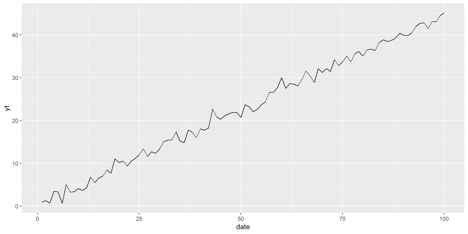
Nonstationary series can have a trend:
- Deterministic: nonrandom function of time:
\(y_t=\mu+\beta t+u_t\) , where \(u_t\) is “iid”
- Example \(\beta=0.45\)
Non-stationary series can have a trend:
Stochastic: random trend, varies over time
Random Walk: \(y_t=b y_{t-1}+\epsilon_t\)
Random Walk with Drift: \(y_t=\mu+y_{t-1}+\epsilon_t\) (as before, \(\epsilon_t\) is iid)
\(\mu\) is the “Drift”;
if \(\mu>0\), then \(y_t\) will be increasing
Question: RW is a special of what process?
Example of a random walk
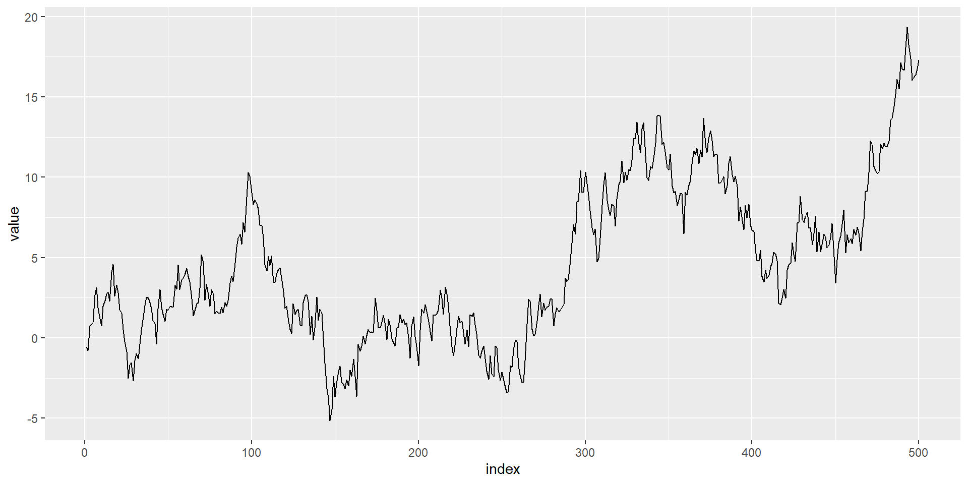
RW with Drift=0.05
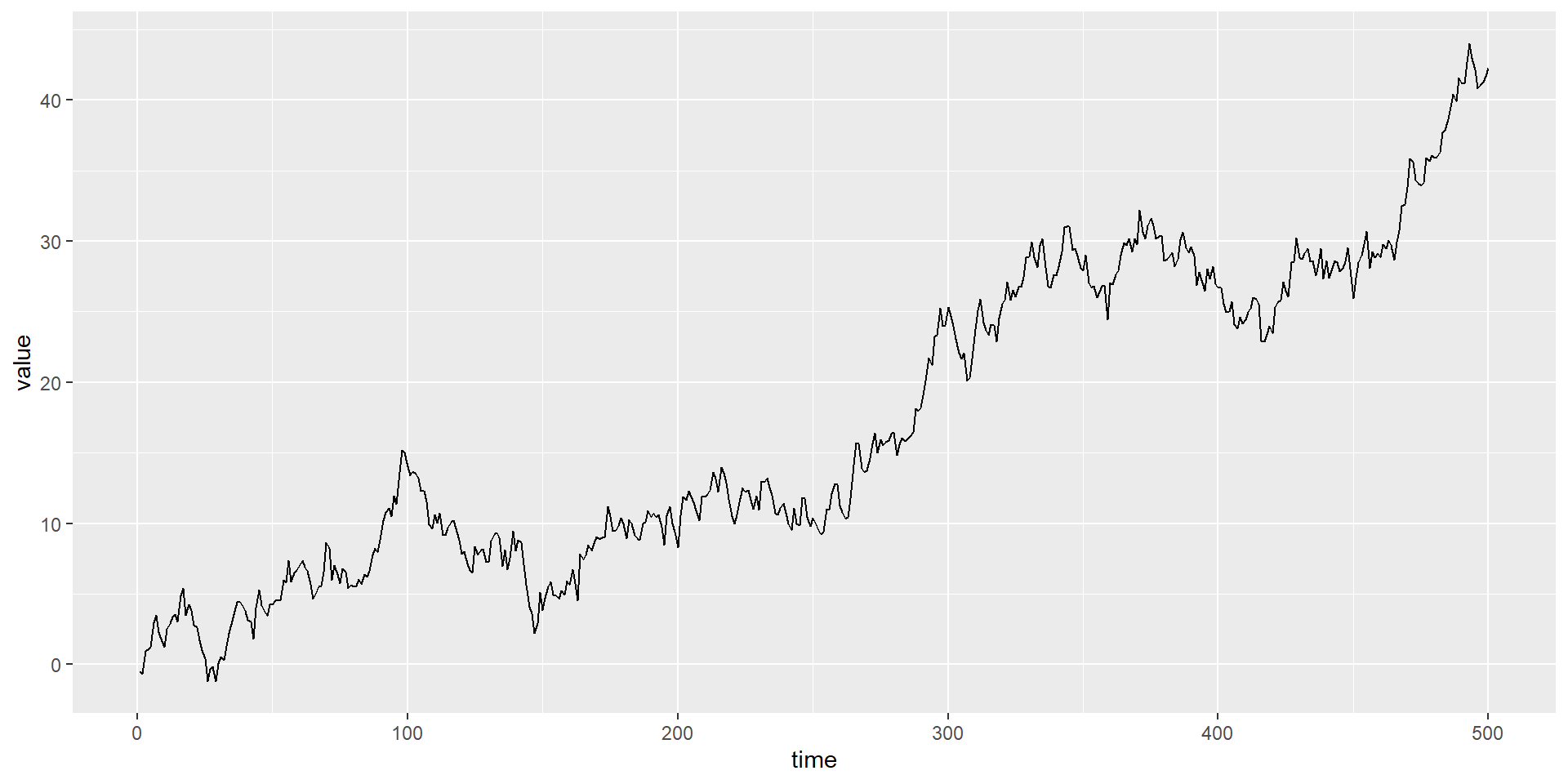
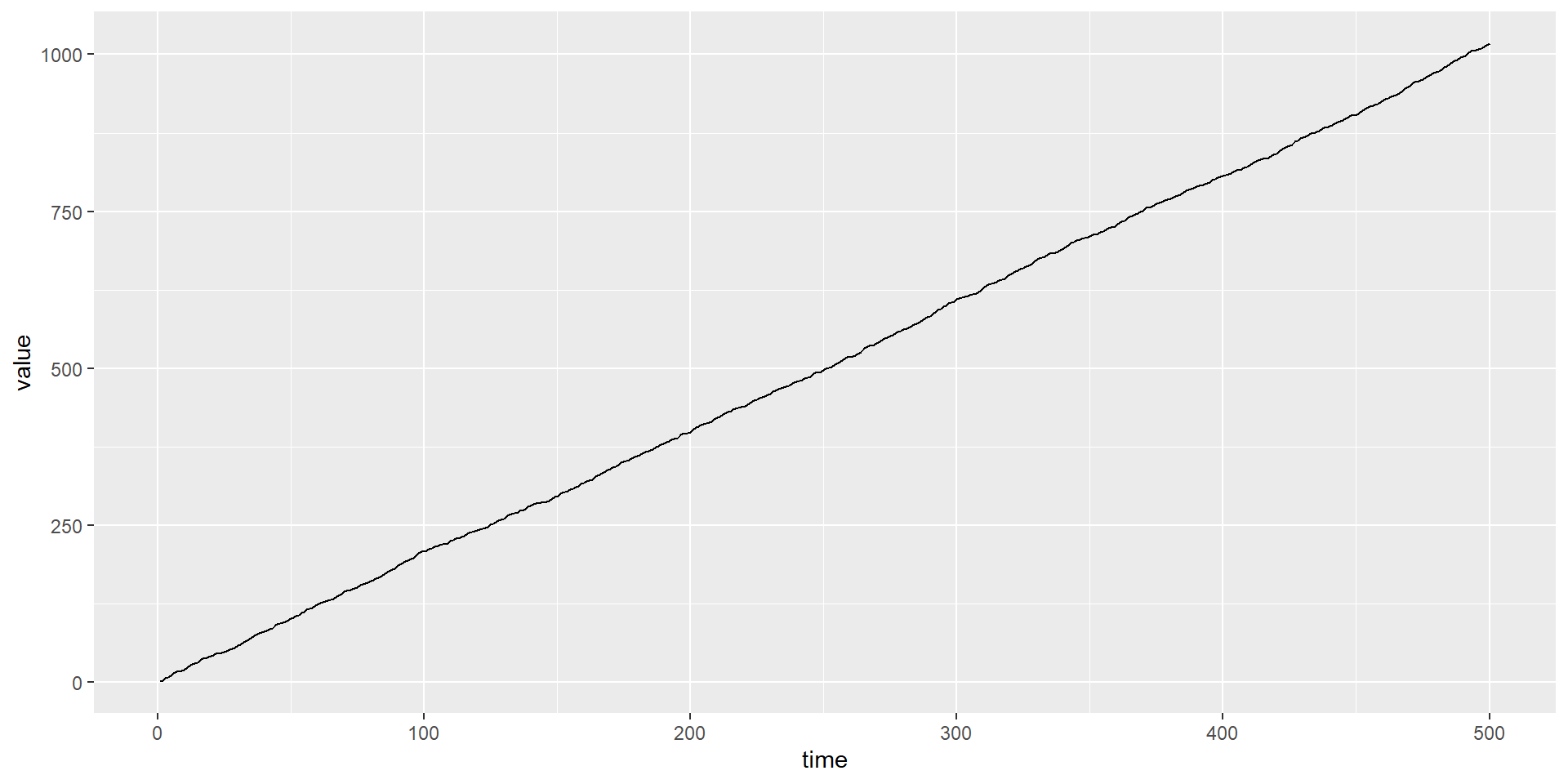
RW with drift is 2
Key Questions:
What is nonstationarity?
Why is it important?
How do we determine whether a time series is nonstationary?
Consequences of non-stationarity
Shocks do not “die out”
Statistical consequences
Non-normal distribution of test statistics
Bias in AR coefficients; poor forecast ability
Shocks do not die out
- Consideer a general AR(1): \(y_t=b y_{t-1}+\epsilon_t\)
- Can be expressed as an MA(q): \(y_t=b^t y_0+\epsilon_t+b\epsilon_{t-1}+b^2\epsilon_{t-2}+. . .+\\b^{t-2}\epsilon_2+b^{t-1}\epsilon_1\)
The impact of shocks (disturbances) will depend on values of \(b\).
\(y_t=b^t y_0+\epsilon_t+b\epsilon_{t-1}+b^2\epsilon_{t-2}+. . .+\\b^{t-2}\epsilon_2+b^{t-1}\epsilon_1\)
Three cases
\(b<0\), \(b^t\) →0 as \(t\) →∞ , so the effects of a shock will diminish as time elapses
\(b=1\), \(b^t=1\) for all t; effect persists, \(y_t=y_0+\sum_{i=1}^{n}\epsilon_{t-i}\) variance grows indefinitely with time.
\(b>1\), shocks become more influential over time.
Statistical consequences of nonstationarity
Non-normal distribution of test statistics
Bias in autorregressive coefficients (b’s);
we might mistakenly estimate an AR(1),
deficient forecast
Usual confidence intervals for coefficients not valid
Statistical consequences of non-stationary for multivariate regressions
For example, two unrelated nonstationary series \(y\) and \(x\) might appear to be related through a standard OLS regression
Hight \(R^2\)
t-statistics that appear to be siginficant
The true test: are the regression residuals stationary? (i-e., long-run equilibrium relationship between \(y\) and \(z\))
Spurious regression practical exercise:
Simulate two random walk series: \(y\) and \(z\) (each with its two disturbances, and either can have drift or not)
- Note by construction, they are unrelated
- Run OLS regression of \(y\) on \(z\), evaluate coefficients, \(R^2\), and plot residulas
Key Questions:
What is nonstationarity?
Why is it important?
How do we determine whether a time series is non- stationary?
Testing for non-stationarity
Recall AR(1) model: \(y_t=by_{t-1}+\epsilon_t\)
Special case: RW, when \(b=1\)
Sationarity requires \(b<1\)
Generalizing to AR(p) :
- Roots of the polynomial below must all be \(>1\) in abs value \(1-b_1Z-b_2Z^2-b_3Z^3-\dots -b_pZ^p\)
If one of the roots=1, then y is said to have a unit root
AR(1) model : \(y_t=by_{t-1}+\epsilon_t\)
Can test for whether \(y\) is a driftless random walk:
\(H_0: b=1\) Or, equaivalently: \(\Delta y_t=\Psi y_{t-1}+\epsilon_t\), \(\Psi=b-1\)
\(H_0: \Psi=0\) - This the ‘Dickey-Fuller’ (DF) test: - Regress \(\Delta y\) on its lag, test for significance of coefficient.
Can extend simple DF test in previous slide:
- Intercept: \(\Delta y_t=\mu+\Psi y_{t-1}+\epsilon_t\)
- Intercept and time trend: \(\Delta y_t=\mu+\Psi y_{t-1}+\alpha t+\epsilon_t\)
- In all three cases, \(H_0:\Psi=0;\) \(y\) has a unit root
Rejecting the unit root test =
find that \(y\) is stationary
Note: critical values for the \(t-statistics\) of \(b\) will vary depending on whether intercept, trend are included.
Some terminology
- Order of integration: number of times a series \(y\) must be differenced to become stationary
- Thus, if \(y\) is “integrated of order zero”, \(I(0)\), then it is stationary (no differencing needed).
- That is, it is stationary in levels
- If \(y\) is \(I(1)\), then its first difference (\(\Delta y\)) is stationary \(\dots\) and so on \(\dots\)
Moving beyond white noise disturbances
DF test assumes that \(\epsilon_t\) is white noise.
However, if \(\epsilon_t\) is autocorrelated, need different version of the test, allowing for higher-order lags:
Augmented Dickey-Fuller (ADF) test:
\(\Delta y_t=\mu+ \gamma y_{t-1}+\sum_i^p \beta_i\Delta y{t-i+1}+\epsilon_t, \gamma=-(1-\sum_i^pb_i)\) and
\(\beta_i=-\sum_i^pb_j\)
ADF test
As with DF, ADF tests whether coefficient on \(y_{t-1}(\gamma)\neq0\)
Must make choices
Intercept, trend, both, none?
p: how many lags? (test statistics are very sensitive to p) - AIC - SBC - General-to-specific (start out with large p, then re-estimate with successively smaller p)
DF, ADF have been found to have low power in certain circumstances:
Stationary processes with near-unit roots
– For example, difficulty distinguishing between \(b = 1\) and \(b = 0.95\) , especially with small samples.
Trend stationary processes
So alternative tests have been designed.
Phillips-Perron (PP) Test:
- Formulation: \(\Delta Y_t=\mu^*+\delta^*t+\Psi y_{t-1}+u_t\) where \(u_t\) is I(0) and may be hetroscedastic and autocorrelated, that is following an ARMA(p,q).
- \(H_0: \Psi=0\)
- PP corrects for any serial correlation and heteroskedasticity in the errors ut by directly modifying the test statistics.
- One advantage of PP: no need to specify lag length.
Kwiatkowski–Phillips–Schmidt–Shin (KPSS)Test:
Null hypothesis: \(y_t\) is trend stationary
Formulation: \(y_t=\beta_0 D_t+\mu_t+u_t\) \(\mu_t=\mu_{t-1}+\epsilon_t\)
Where \(D_t\) contains deterministic components (constant or constant plus time trend), \(\mu_t\) is a random walk
\(H_0: \sigma_{\epsilon}^2=0\)
\(H_1: \sigma_{\epsilon}^2>0\)
KPSS critical values are obtained by simulation methods.
A few notes: A few notes: - DF, ADF, and PP are called “unit root tests”; the null hypothesis is that yt has a unit root; is I(1) or higher.
KPSS, on the other hand, is a “stationarity test”, null hypothesis is that yt is I(0).
Correct specification is key: intercept and trend should be included when appropriate.
Structural breaks can complicate matters further.
A unified way of looking at the unit root tests Slightly different representation: \(y_t=\mu+\alpha t+ u_t\) \(u_t=\rho u_{t-1}+\epsilon_t\)
\(H_0: =1\) y has a unit root
\(H_1: |\rho|<1\) y is stationary
- If \(\epsilon_t\) is white noise, then DF can be used
- If \(\epsilon_t\) is ARMA(p,q) then use ADF or PP
Simulate three processes:
Stationary process with near-unit roots
Trend stationary process
An I(1) process
Graph them and observe their behavior
Conduct Unit Root/Stationarity Tests on all three.
In “Simulated Times Series Examples.xlsx”
Simulate an I(0) process with a structural break
Import into R
Graph and observe
Conduct Unit Root/Stationarity Tests
Now let’s work with real world data
Choose a series:
Look at graph and correlogram for a specific time series
Does it appear to be non-stationary? Does it appear to have a trend, or a structural break?
Undertake Unit Root/Stationarity Tests
Do the different tests agree?
If you suspect a structural break, re-test for two sub-samples