Beautiful Presentations and Reports with Quarto in R

Zahid Asghar

2026-09-12

Cement Production

We have data from Cement Manufacturers Association. Lets explore this data as follows:

library(tidyverse)
library(lubridate)
library(readr)
library(readxl)
library(collapse)
library(kableExtra)
library(dynlm)
library(forecast)
library(stargazer)
library(scales)
library(xts)
library(urca)
library(tsibble)
library(fpp2)
library(fpp3)
library(ggthemes)
library(DT)
library(fable)
library(fabletools)

Read data

library(readr) # To load data from csv file, if one needs to load data from excel, then use excel file
cement<-read_csv("data/cement.csv")
glimpse(cement)
## Rows: 1,116
## Columns: 6
## $ Date                         <chr> "07/1991", "07/1991", "07/1991", "08…
## $ `Series Name`                <chr> "Total Cement Sales", "Domestic Ceme…
## $ Output                       <dbl> 599, 599, NA, 632, 632, NA, 633, 633…
## $ Unit                         <chr> "Thousand Metric Ton", "Thousand Met…
## $ `Observation Status`         <chr> "Normal", "Normal", "Missing value",…
## $ `Observation Status Comment` <lgl> NA, NA, NA, NA, NA, NA, NA, NA, NA, …

Selecting and Renaming variables

cement<-cement %>% rename(Category=`Series Name` )

#cement<-ts(cement, frequency = 12, start=c(1991,7))
#cement
#cement<-cement %>% mutate(Month=yearmonth(Date)) %>% as_tsibble(index = Month)

cement<-cement %>% filter(Category=="Total Cement Sales") # Select only Total Cement Sales

cement$Date<-my(cement$Date) # Formating required
cement$Date<-as_date(cement$Date,format="%Y-%m")

#cement<-tsibble(cement)
cement

cement$year<-year(cement$Date)
cement

cement_yrly<-cement %>% group_by(year) %>% summarise(prod_yr=sum(Output))
cement_yrly<-cement_yrly %>% filter(year<=2021)
#cement_yrly$year<-make_date(cement_yrly$year)
#cement_yrly<-tsibble(cement_yrly)
cement_yrly

#cement<-tsibble(cement)

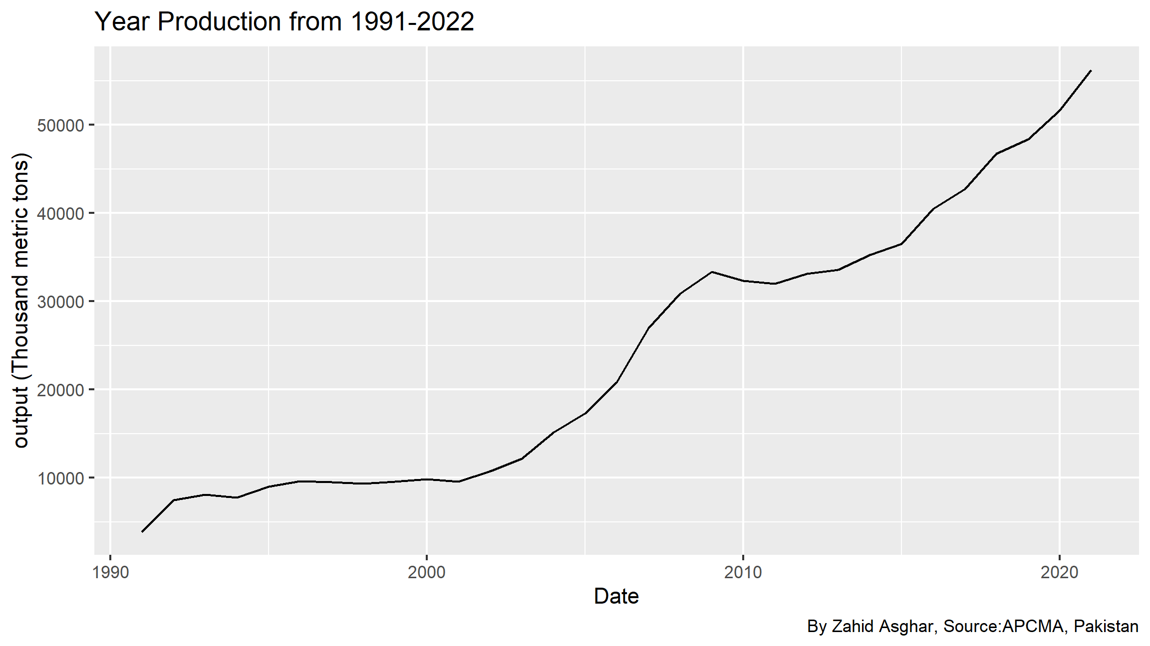
Annual cement sale

What happens if year 2022 is included?

Why annual is less informative?

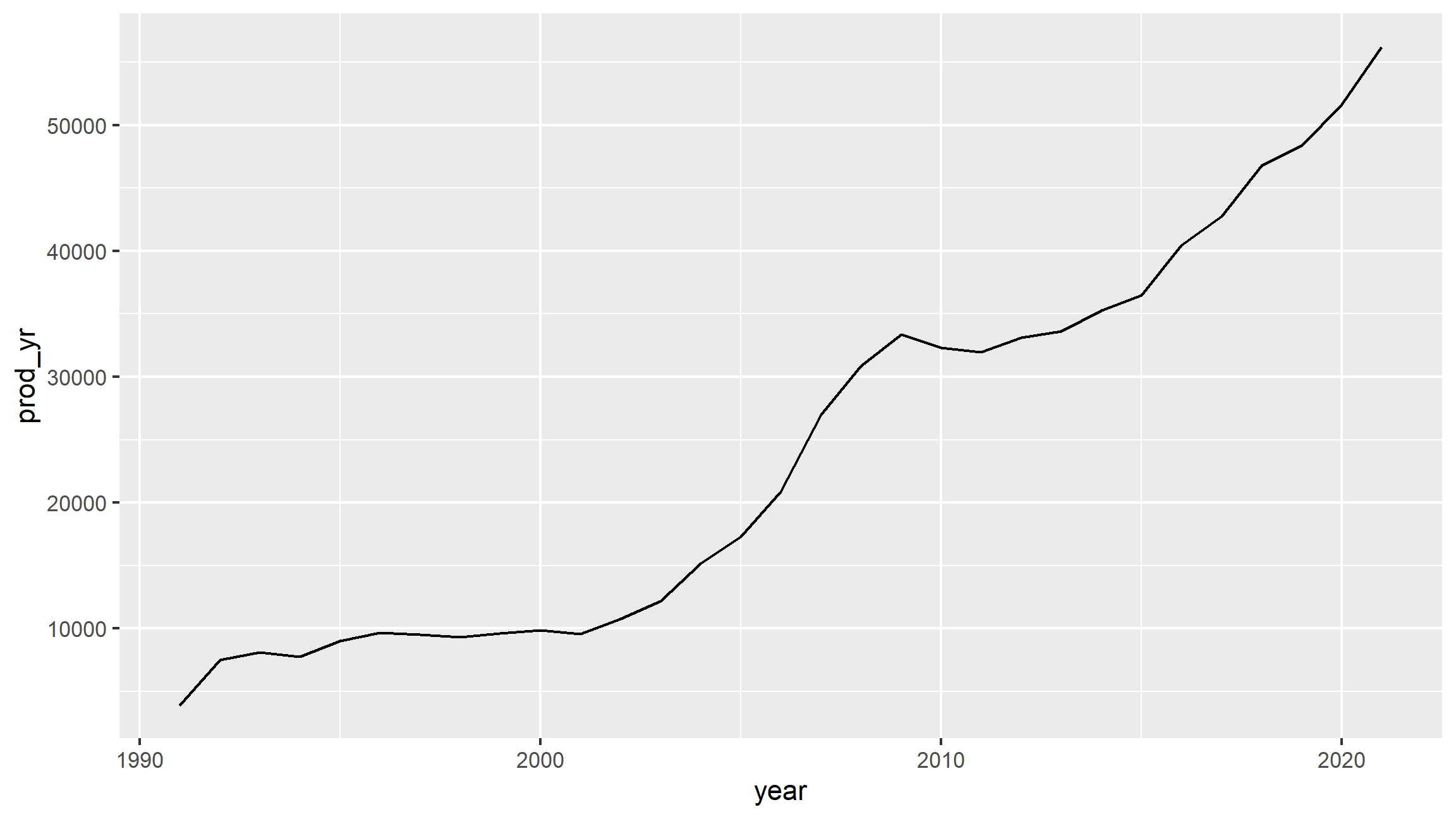
p1<-ggplot(cement_yrly)+aes(x=year,y=prod_yr)+geom_line()
p1

#forecast::naive(cement_yrly$prod_yr, h=4) %>% autoplot() 

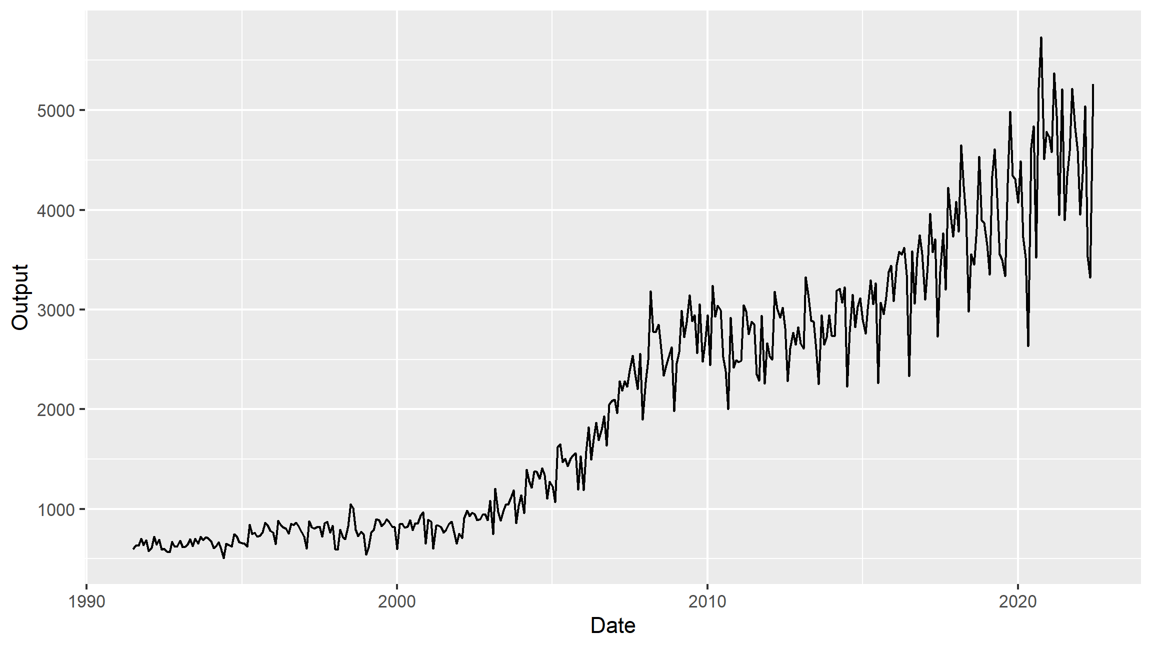
Monthly cement production

pm<-ggplot(cement)+aes(x=Date,y=Output)+geom_line()
pm

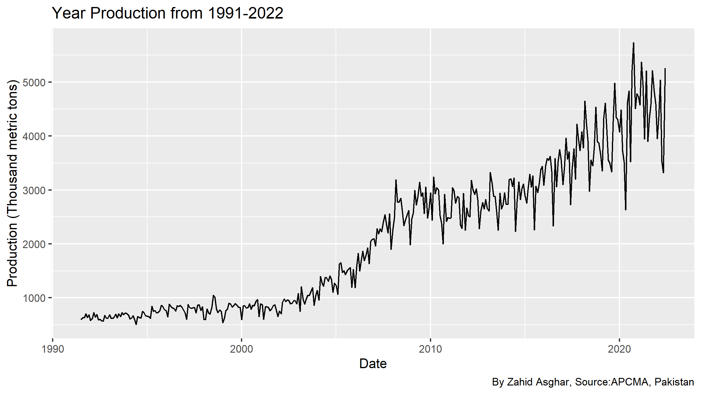
Labels, data source, theme

p1+labs(x="Date",y="output (Thousand metric tons)", title = "Year Production from 1991-2022", caption = "By Zahid Asghar, Source:APCMA, Pakistan")

pm+labs(x="Date",y="Production (Thousand metric tons)", title = "Year Production from 1991-2022", caption = "By Zahid Asghar, Source:APCMA, Pakistan")

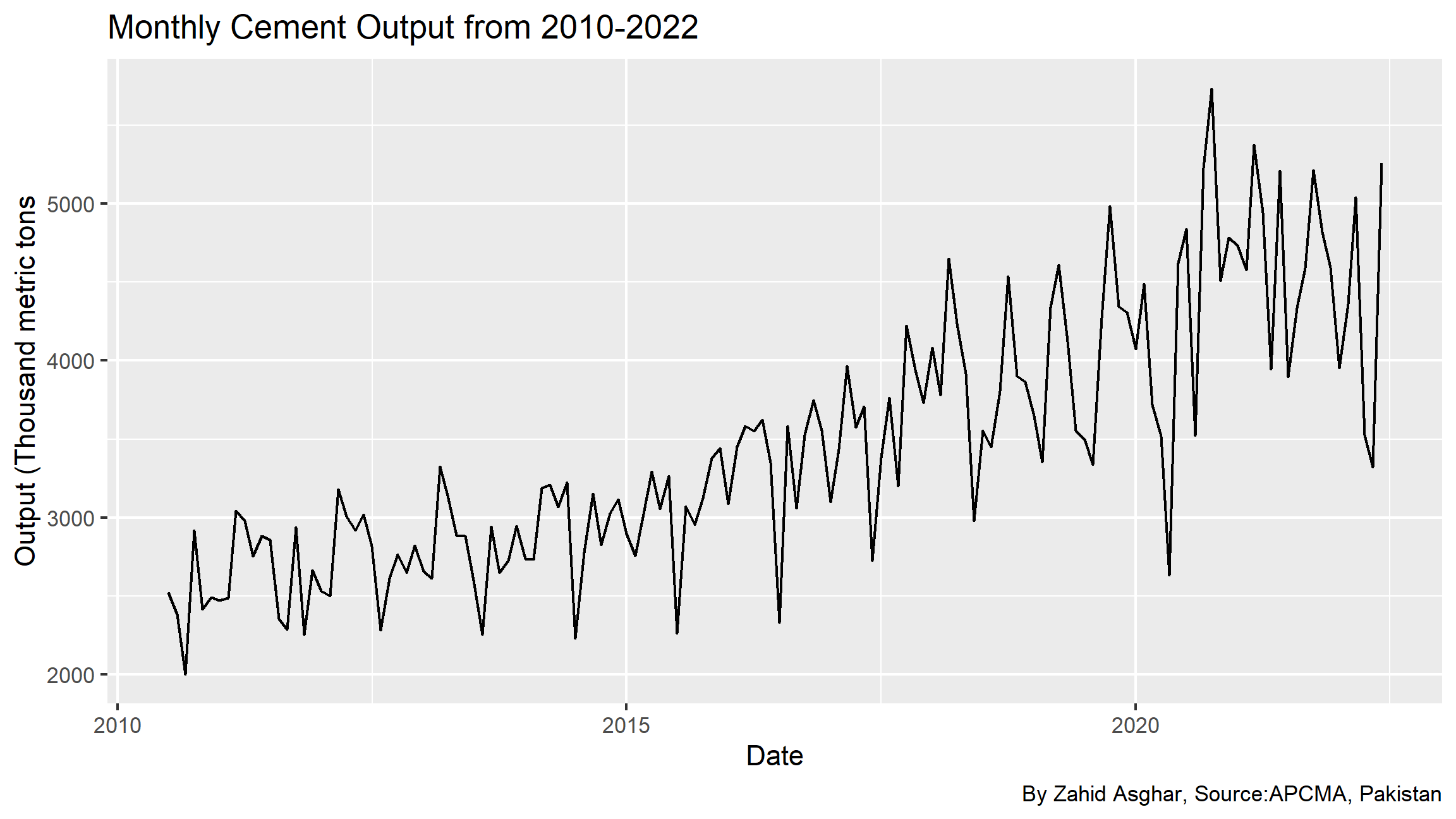
Last 10 years data

cement_2010<-cement %>% filter(Date>="2010-6-30")
cement_2010

p11<-ggplot(cement_2010)+aes(x=Date,y=Output)+geom_line()
p11+labs(x="Date",y="Output (Thousand metric tons", title = "Monthly Cement Output from 2010-2022", caption = "By Zahid Asghar, Source:APCMA, Pakistan")

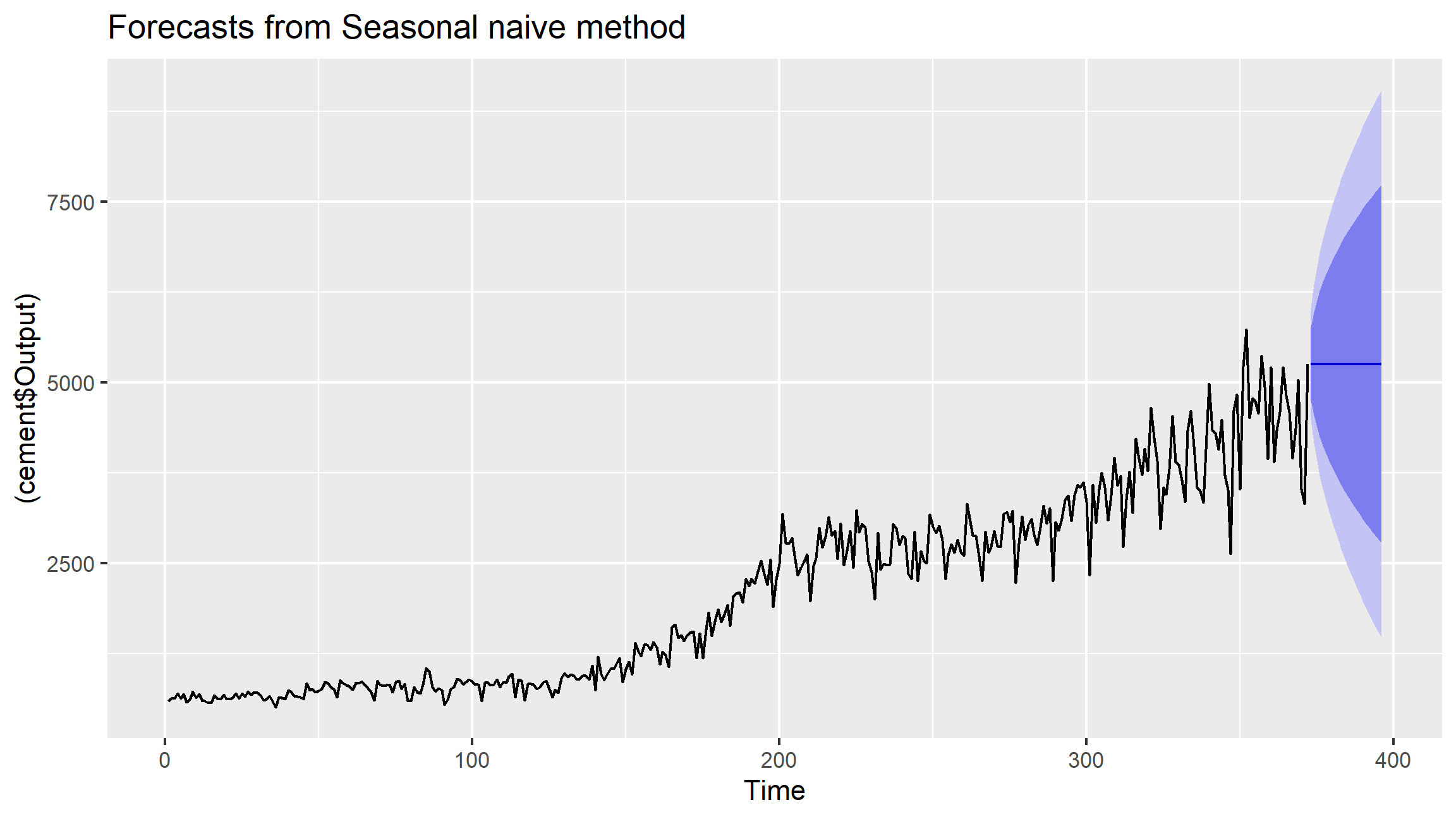
Forecasting

forecast::snaive((cement$Output), h = 24) %>% autoplot()

ARIMA models

## Series: cement$Output 
## ARIMA(4,1,1) with drift 
## 
## Coefficients:
##         ar1     ar2    ar3     ar4    ma1  drift
##       0.137  -0.106  0.082  -0.169  -0.83  10.54
## s.e.  0.064   0.059  0.059   0.057   0.04   2.67
## 
## sigma^2 = 100902:  log likelihood = -2661
## AIC=5337   AICc=5337   BIC=5364
## 
## Training set error measures:
##                  ME RMSE MAE   MPE MAPE  MASE     ACF1
## Training set -0.403  315 202 -2.99 10.1 0.811 -0.00574

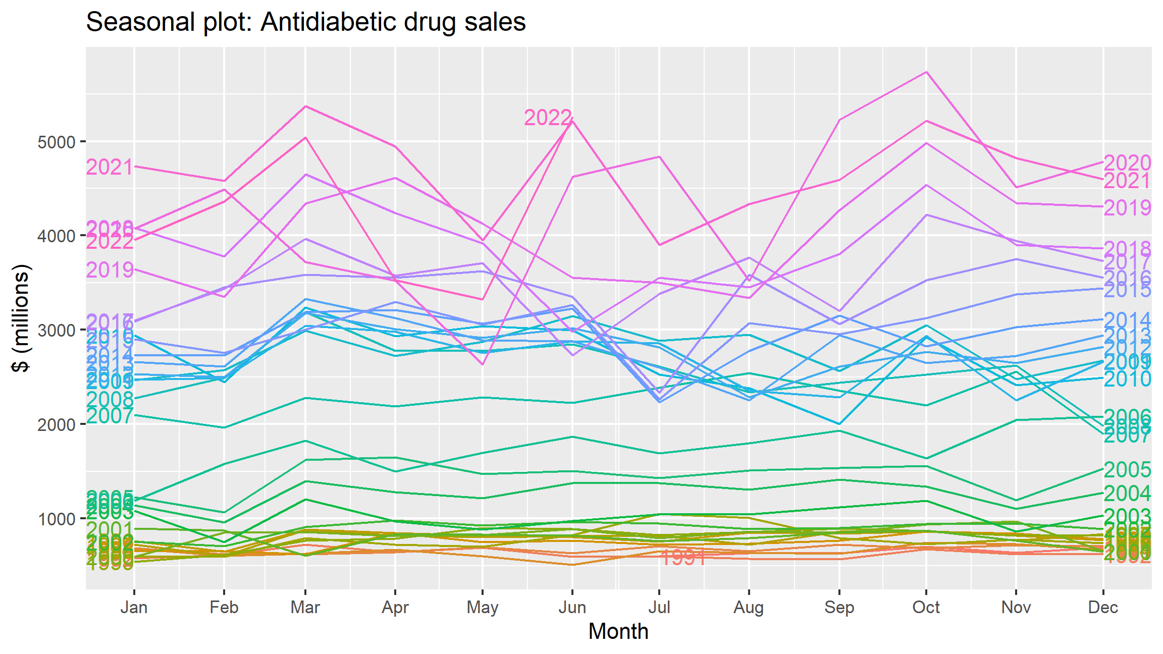
Seasonal Plot

cement<-cement %>% mutate(Month=yearmonth(Date)) %>% as_tsibble(index=Month)

cement %>%
  gg_season(Output,labels = "both")+
  labs(y = "$ (millions)",
       title = "Seasonal plot: Antidiabetic drug sales")

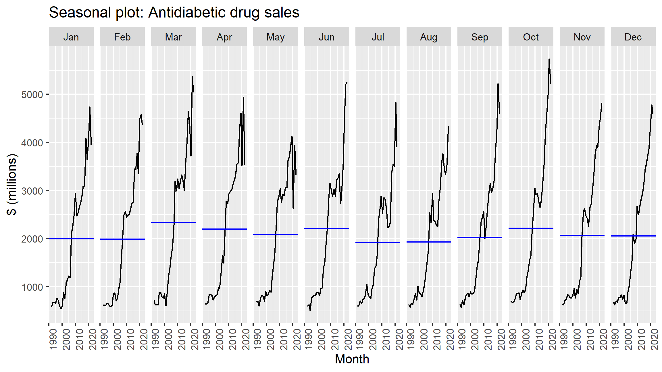
Monthly Analysis

cement %>%
  gg_subseries(Output,labels = "both")+
  labs(y = "$ (millions)",
       title = "Seasonal plot: Antidiabetic drug sales")

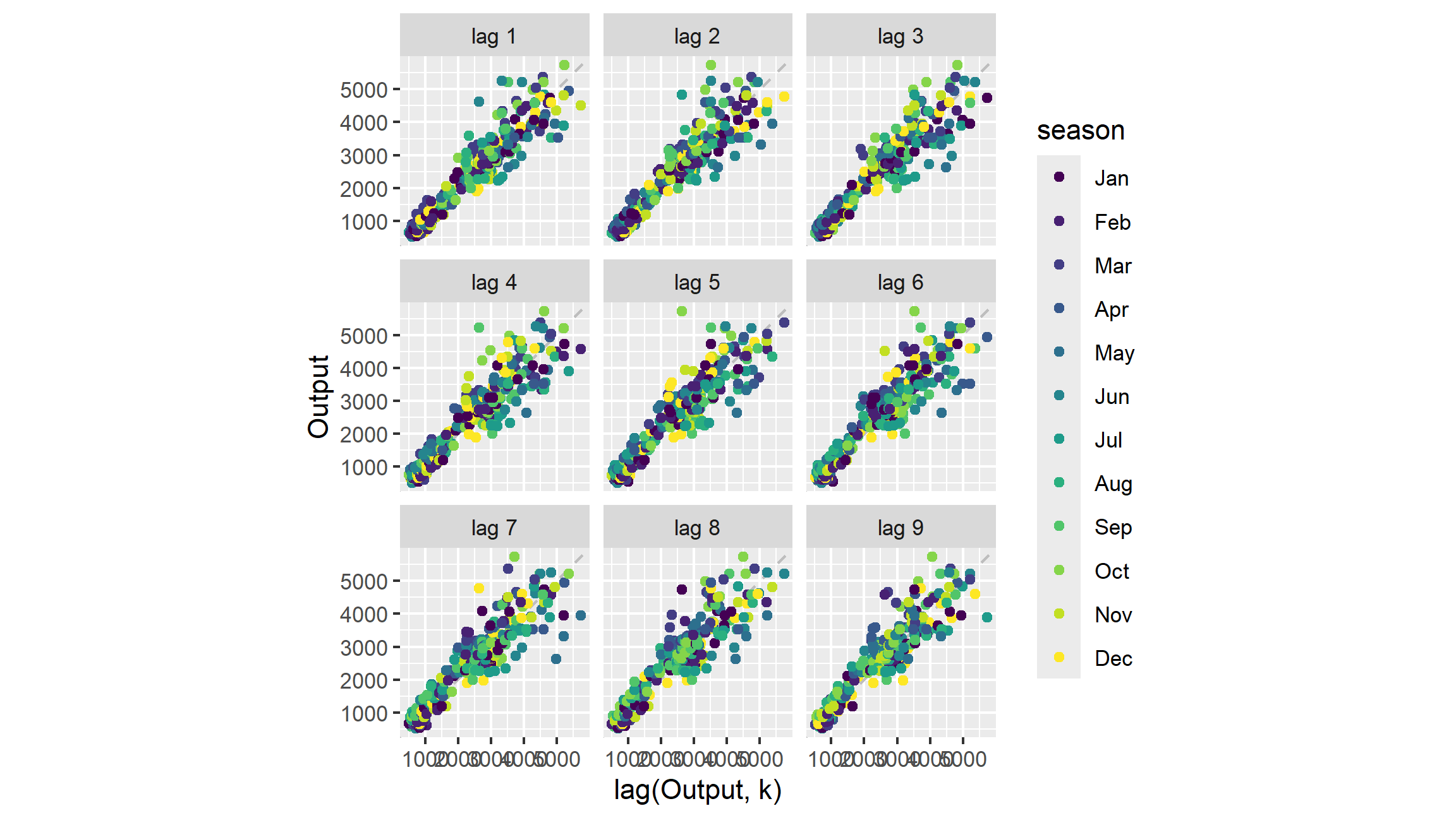
Lag Plots

cement %>%
  gg_lag(Output, geom = "point") +
  labs(x = "lag(Output, k)")

Shiny Interactive View

library(seasonalview)
library(shiny)
#cement_prod<-ts(data = cement$Output,frequency = 12, start=c(1991,7))
#view(seas(cement_prod))

quarto render cement.qmd --to pdf