Sationary and Nonstationary Series
Macroeconomic Forecasting Lecture
2025-03-04
Properties of Time Series
Outline
Part 1 : Stationary processes
- Identification
- Estimation & Model Selection
- Putting it all together
Part 2: Nonstationary processes
Characterization
Testing
Univariate Analysis
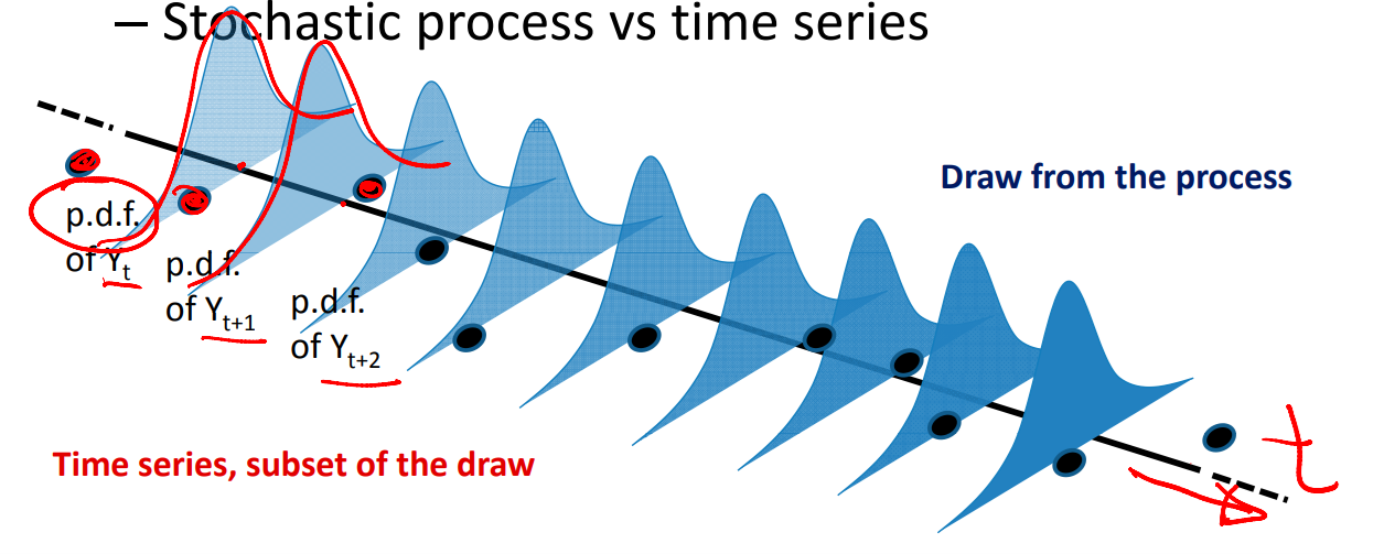
Each distribution is a draw from a random process.
Strong statinarity
- Strong statinarity vs weak stationarity (covariance stationarity)
- Strong stationarity:
- Same distribution over time
- Same covariance structure over time But its only a theoretical concept. In practice, we use covariance stationarity.
- Covariance stationary:
- Unconditional mean \(E(Y_t)=E(Y_{t+j})=\mu\)
- variance constant \(Var(Y_t)=Var(Y_{t+j})=\sigma^2_y\) and
- Covariance depends on time j that has elapsed between observations, not on reference period \(Cov(Y_t,Y_{t+j})=Cov(Y_s,Y_{s+j})=\gamma_j\)
- Unconditional mean \(E(Y_t)=E(Y_{t+j})=\mu\)
- Strong stationarity:
Part1 : Stationary Process
Just to remind you….
- Identification
- Estimation & Model Selection
- Putting it all together
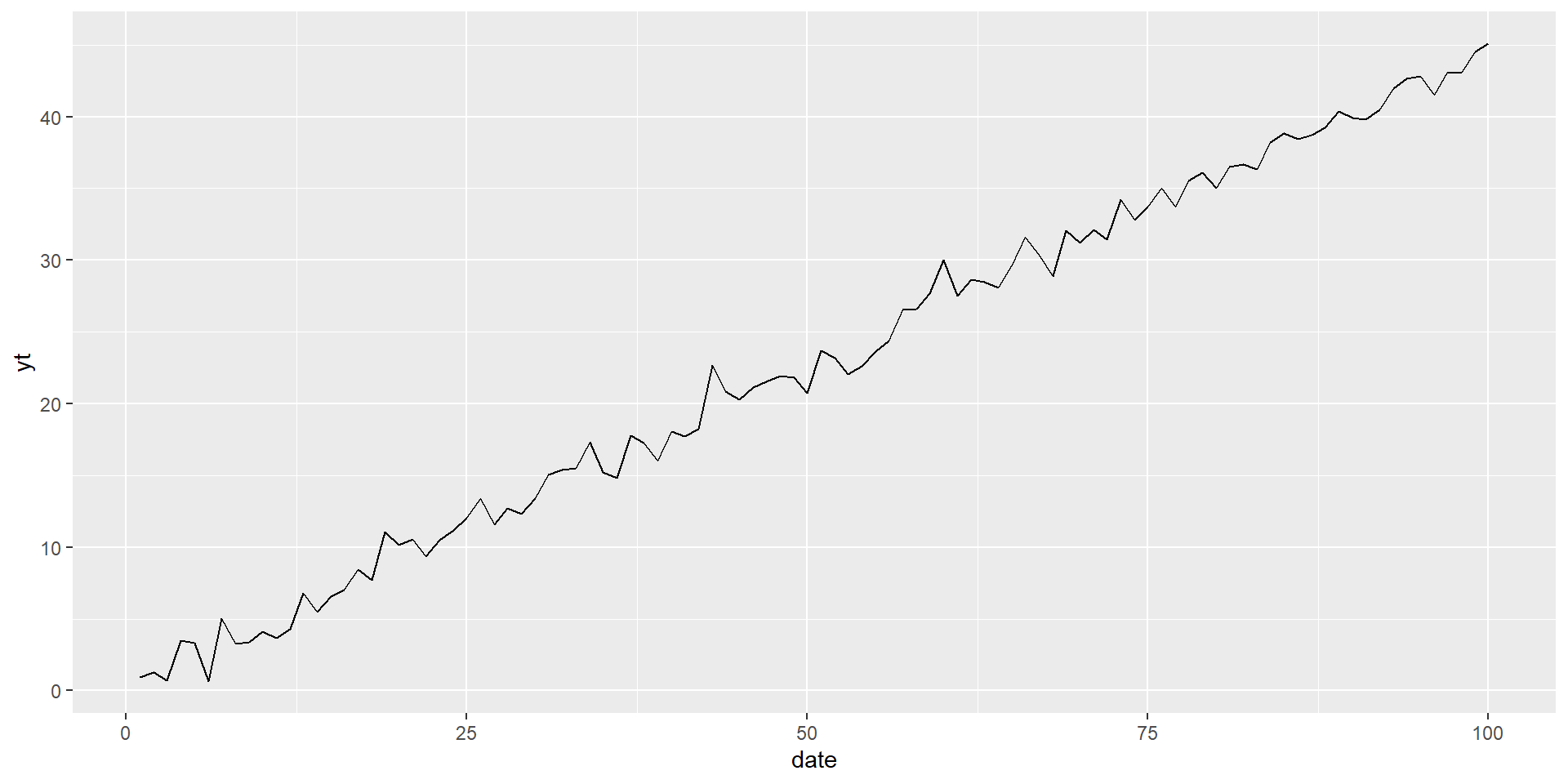
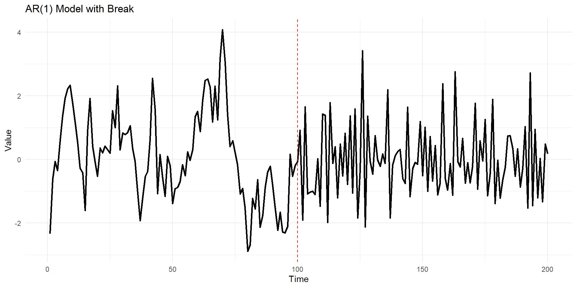
The first step is visual inspection: graph and observe your data.
“You can observe a lot just by watching” Yogi Berra
Plot plot and plot your data

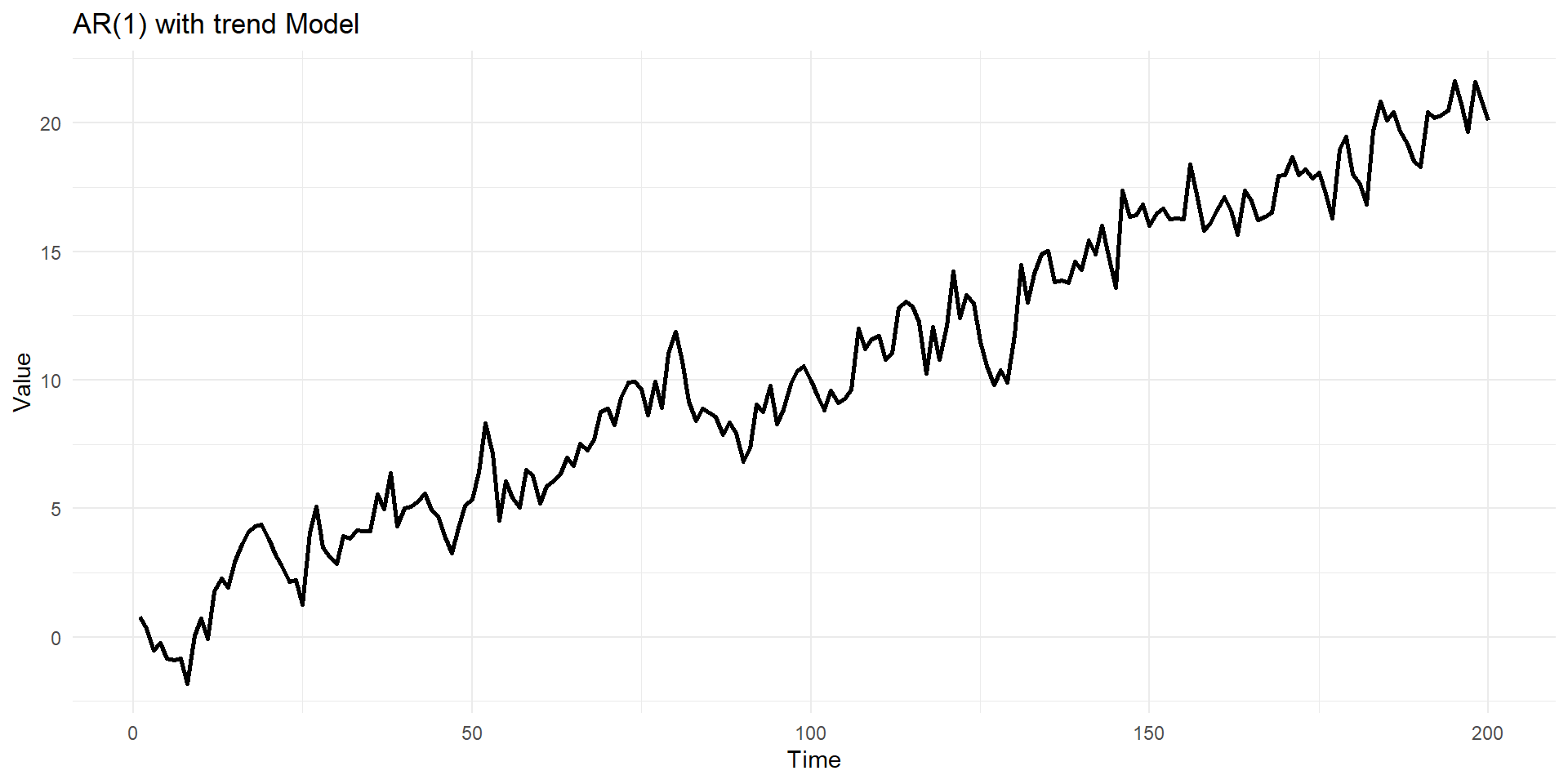
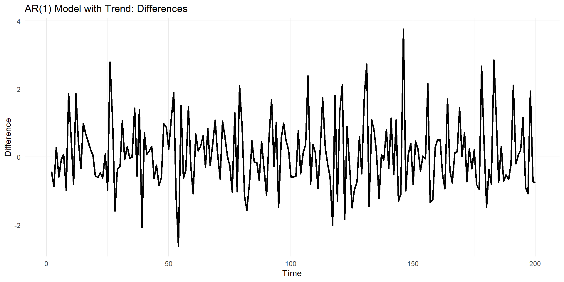
Differenced model of trend variable (third case)
Difference can remove the trend.
\(y_t^{*}=y_t-y_{t-1}\)
Identification
Assuming that the process is stationary, there are three basic types that interest us:
Autoregressive (process) \(y_t=a+b_1y_{t-1}+b_2y_{t-2}+...+b_py_{t-p}+\epsilon_t\)
Moving Average : MA(process) : \(y_t=\mu+\phi_1\epsilon_{t-1}+\phi_2\epsilon_{t-1}+...+\phi_q\epsilon_{t-1}+\epsilon_t\)
Combined ARMA-process \(y_t=a+b_1y_{t-1}+b_2y_{t-2}+...+b_py_{t-p}+\\\phi_1\epsilon_{t-1}+\phi_2\epsilon_{t-1}+...+\phi_q\epsilon_{t-1}+\epsilon_t\)
Some notation: AR(p), MA(q), ARMA(p,q), where p,q refer to the order (maximum lag) of the process
\(\epsilon_t\) is a white noise disturbance:
\(E(\epsilon_t=0)\), \(Var(\epsilon_t=\sigma^2)\) , \(Cov(\epsilon_t,\epsilon_s=0 , if \ t\neq s)\)
Tools for Identification
Where are we? Where are we going?
Stationary process (visual inspection) y
Learned about possible processes for y
Need to identify which one in order to understand, then eventually forecast y
tools to help identify
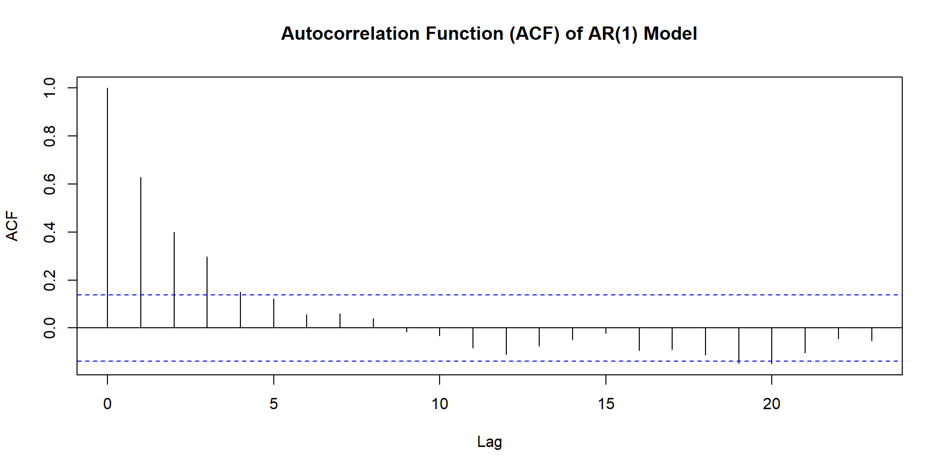
Autocovariance and autocorrelation relations between observations at different lags:
- Autocovariance \(\gamma_j=E[(y_t-\mu)(y_{t-j}-\mu)]\)
- Autocorrelation \(\rho_j=\gamma_j / \gamma_0\)
- ACF or Correlogram : graph of autocorrelations at each lag
NULL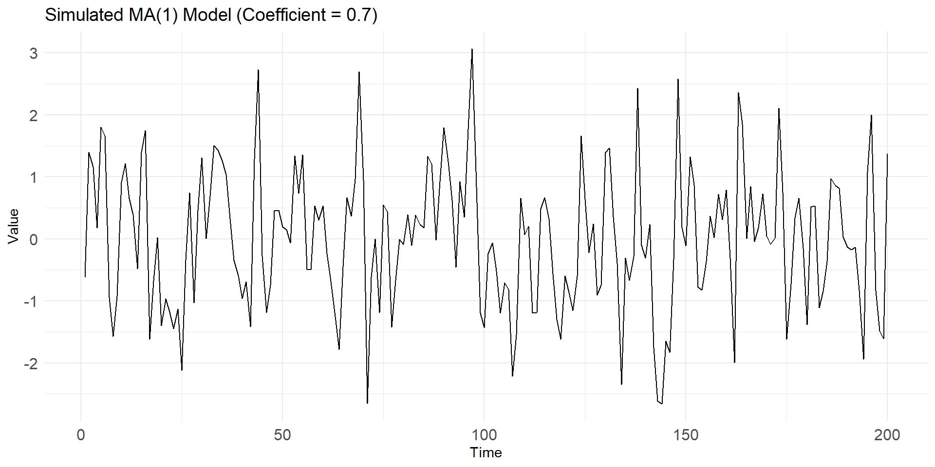

NULL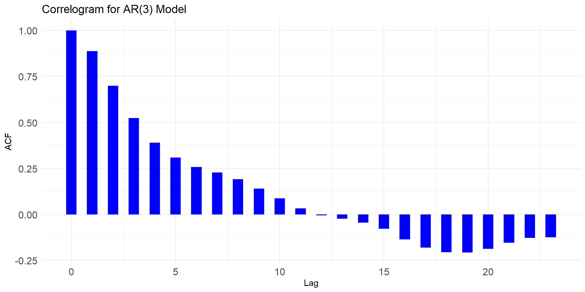
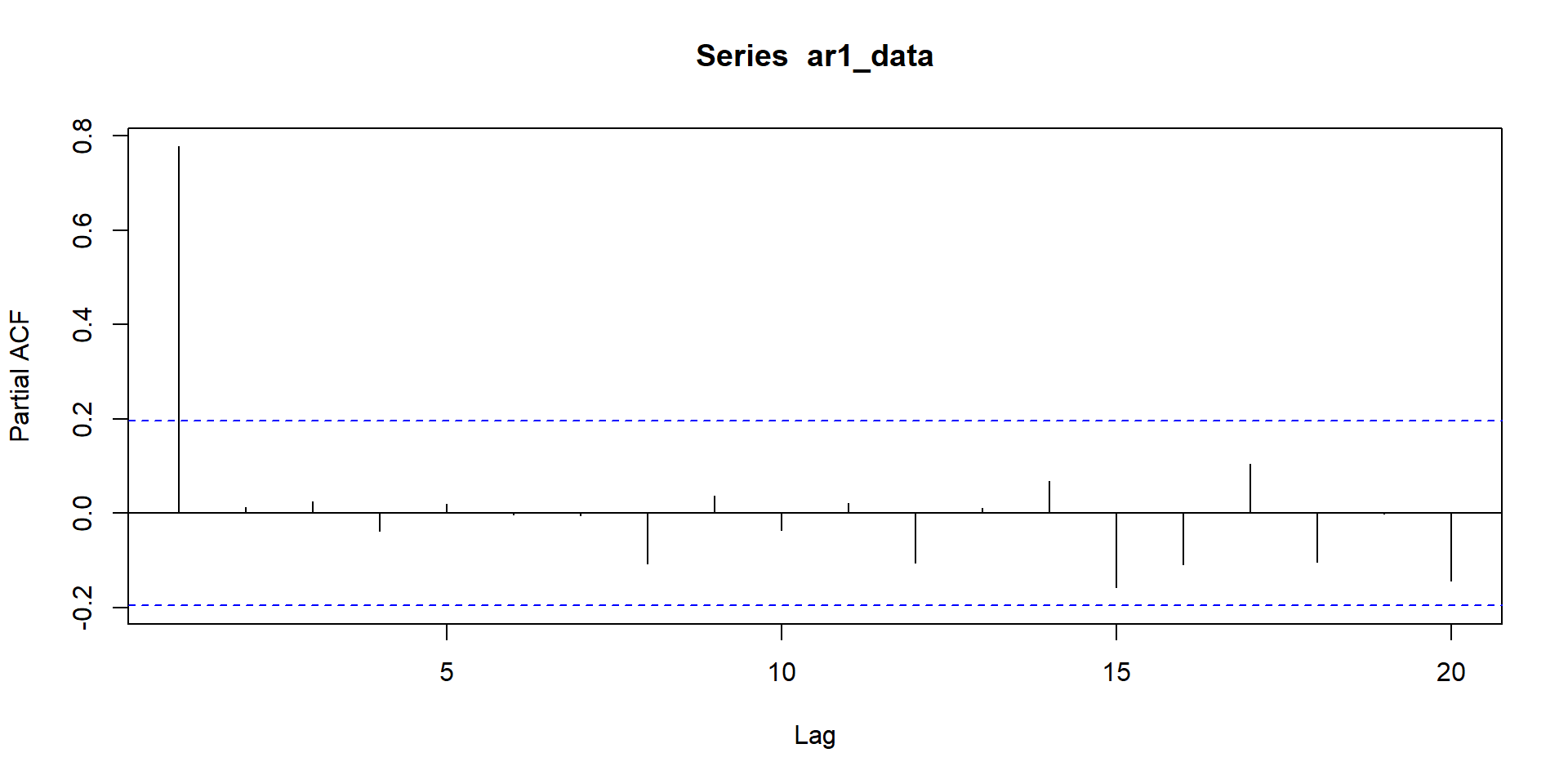
Patterns for PACF
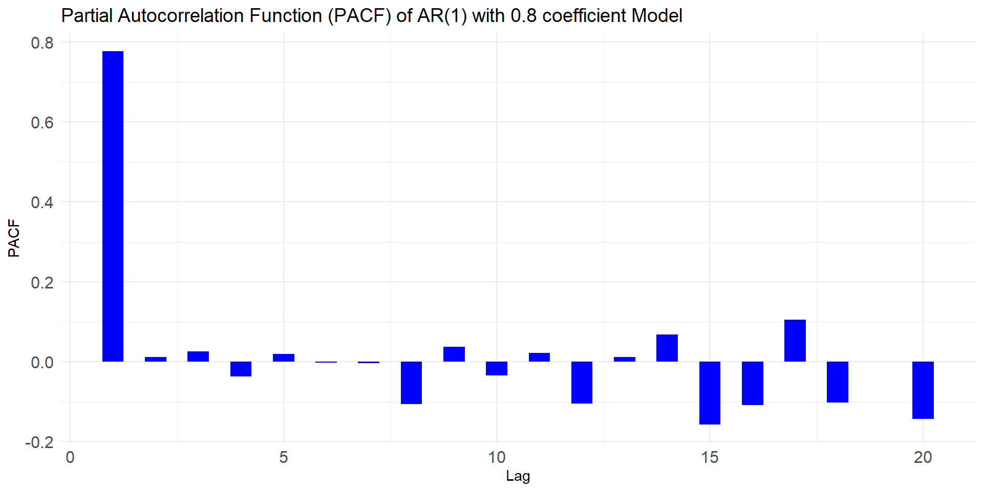
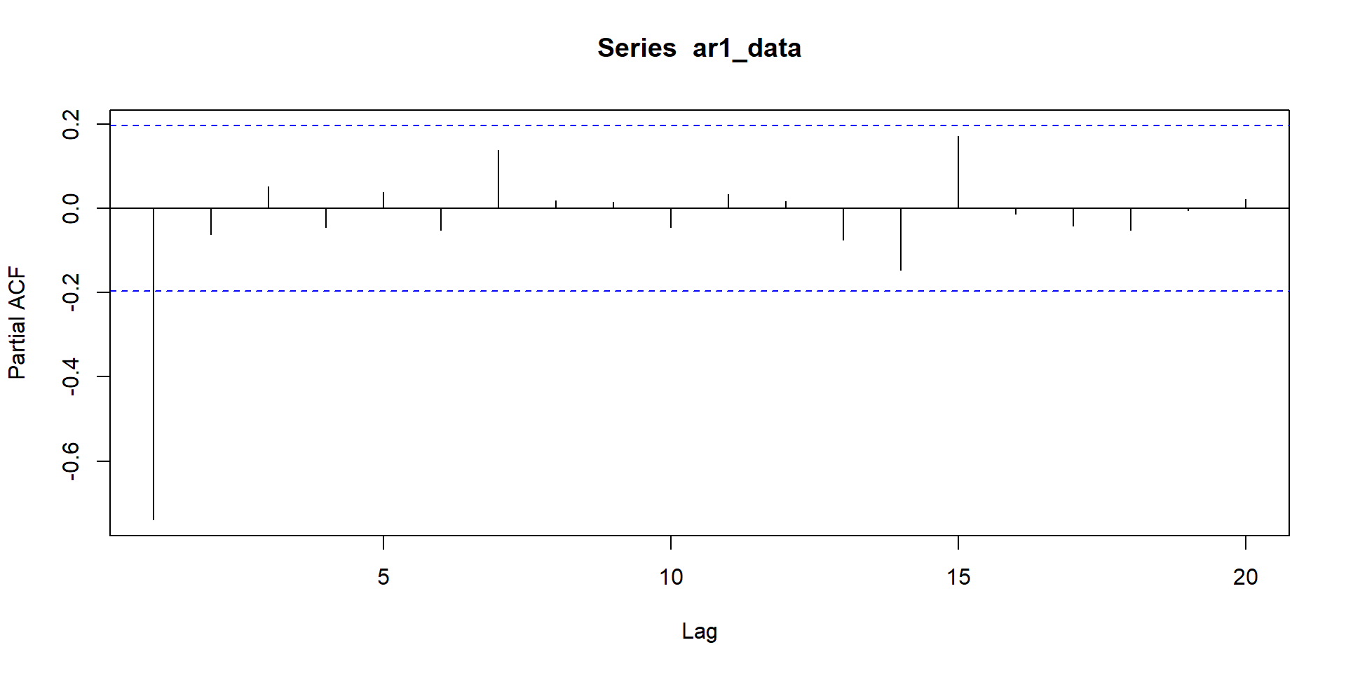

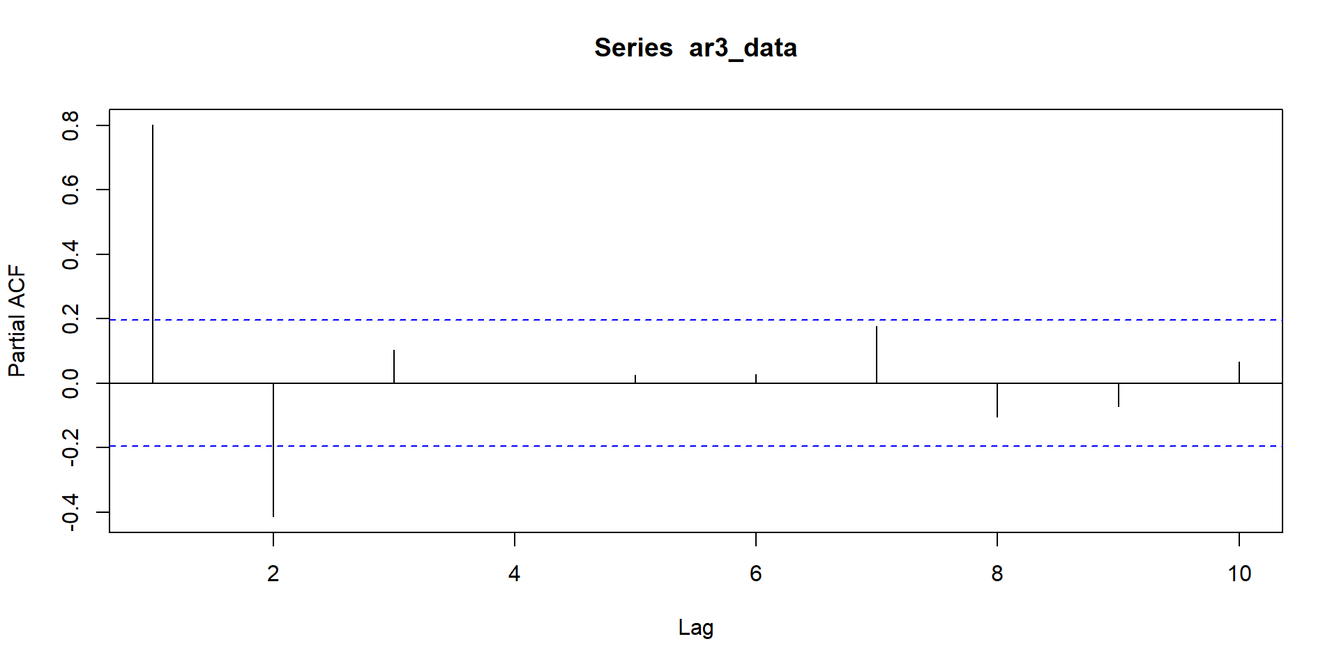
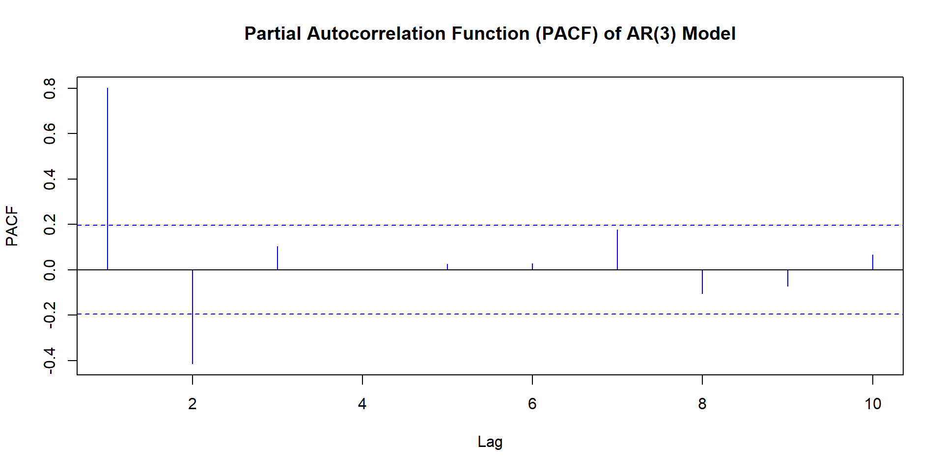
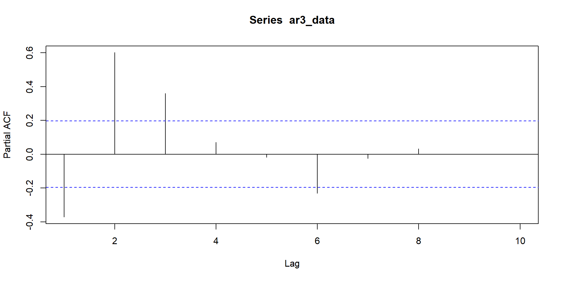

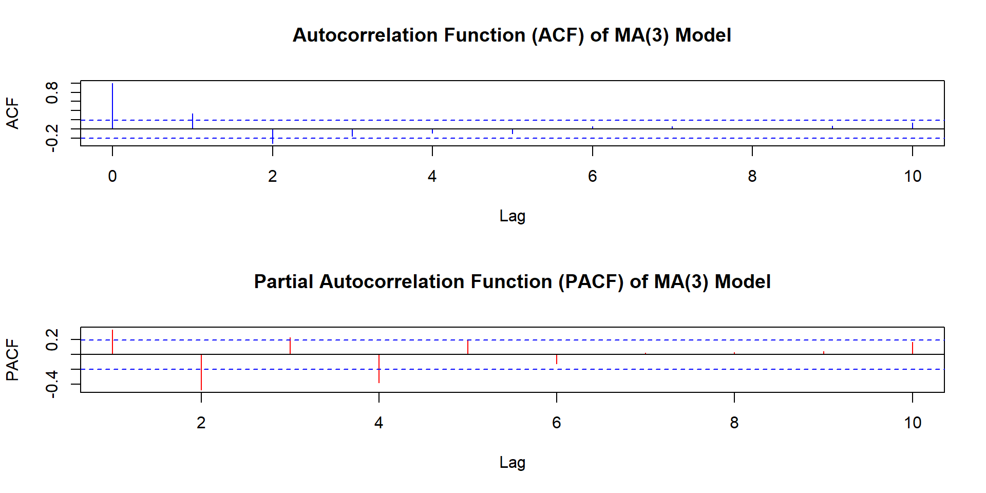
ACF and PACF for MA(3)
Stationary Time Series
We now have a tool (ACF, PACF) to help us identify the stochastic stochastic process underlying time series we are observing. Now we will: - Summarize the basic patterns to look for - Observe an actual data series and make an initial guess Observe an actual data series and make an initial guess
- Next step: estimate (several alternatives) based on this guess
Summary Table Pattern
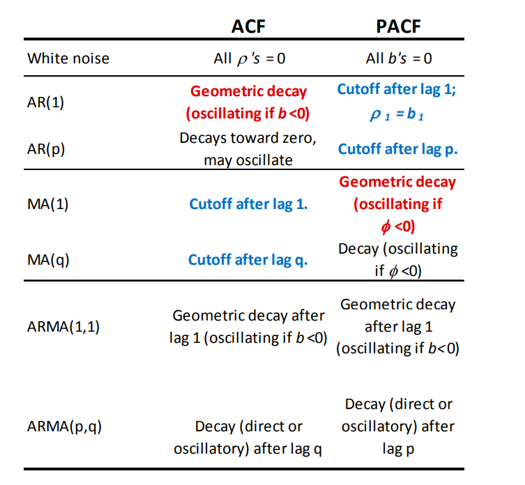
Pattern for model identification
Tips
ACF’s that do not go to zero could be sign of nonstationarity
ACF of both AR, ARMA decay gradually, drops to 0 for MA
PACF decays gradually for ARMA, MA, drops to 0 for AR
Possible approach: begin with parsimonious low order AR, check residuals to decide on possible MA terms.
When looking at ACF, PACF
- Box-Jenkins provide sampling variance of the observed ACF and PACFs (\(r_s\) and \(b_s\))
- Permits one to construct confidence intervals around each → assess whether significantly \(\neq0\)
- Computer packages provide this automatically
Estimation and Model Selection
- Decide on plausible alternative specifications (ARMA)
- Estimate each specification
- Choose “best” model, based on:
- Significance of coefficients
- Fit vs parsimony (criteria)
- White noise residuals
- Ability to forecast
- Account for possible structural breaks
Fit vs parsimony (information criteria):
- Additional parameters (lags) automatically improve fit but reduce forecast quality
- Tradeoff between fit and parsimony; widely used criteria:
- Akaike Information Criterion (AIC) \(AIC=T ln(SST)+2(p+q+1)\)
- Schwartz Bayesian Criterion (BIC) \(SBC= T ln(SST)+(p+q+1)ln(T)\)
- SBC is considered to be preferable for having more parsimonious models than AIC
White noise errors :
Aim to eliminate autocorrelation in the residuals (could indicate that model does not reflect the lag structure well)
Plot “standardized residuals” (\(\epsilon_{it}\) ) No more than 5% of them should lie outside [-2,+2] over all periods
Look at \(r_s\), \(b_s\) (and significance) at different lags Box-Pierce Statistic: joint significance test up to lag \(s\): \(\bar{x} = \frac{1}{n}\)
\(Q=T \sum_{k=1}^{s} r_k^2\)
\(H_0\) : all \(r_k=0\), \(H_1\): at least one \(r_k\neq0\)
\(Q\) is distributed as \(\chi^2(s)\) under \(H_0\)
Forecastability
Can assess how well the model forecasts ” out of sample”:
- Estimate the model for a sub-sample (for example, the first 250 out of 300 observations).
- Use estimated parameters to forecast for the rest of the sample (last 50)
- Compute the ” forecast errors” and assess:
- Mean Squared Prediction Error
- Granger-Newbold Test
- Diebold-Mariano Test
Account for possible structural breaks:
- Does the same model apply equally well to the entire sample, or do parameters change (significantly) within the sample?
How to approach:
Own priors/suspicion : Chow test for parameter change
If priors not strong, recursive estimation, tests for parameter stability over the sample, for example, CUSUM
Learning all above with simulated data
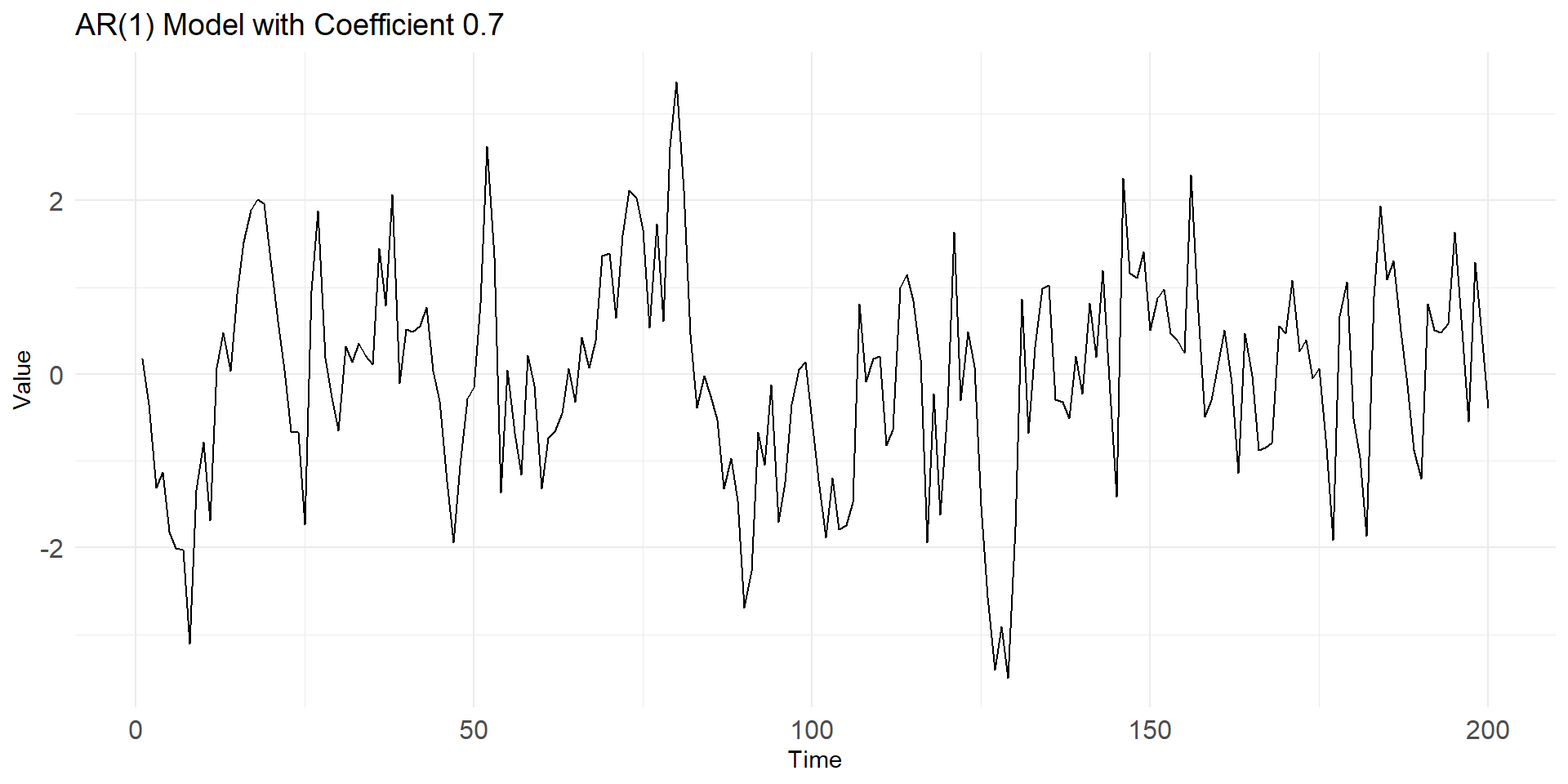
Lets simulate MA(1), AR(1) series in R
# Set the parameters
mu <- 0       # Mean of the series
theta <- 0.6  # Moving average coefficient
n <- 200      # Number of time points

# Simulate data from the MA(1) model
set.seed(123)  # For reproducibility
ma1_data <- arima.sim(model = list(ma = theta), n = n, mean = mu)

# Create a data frame with time series data
time_series_data <- data.frame(Time = 1:n, Value = ma1_data)

# Create a ggplot2 line plot
ggplot(time_series_data, aes(x = Time, y = Value)) +
  geom_line(linewidth=1) +labs(title = "MA(1) Model ", x = "Time", y = "Value") +
  theme_minimal()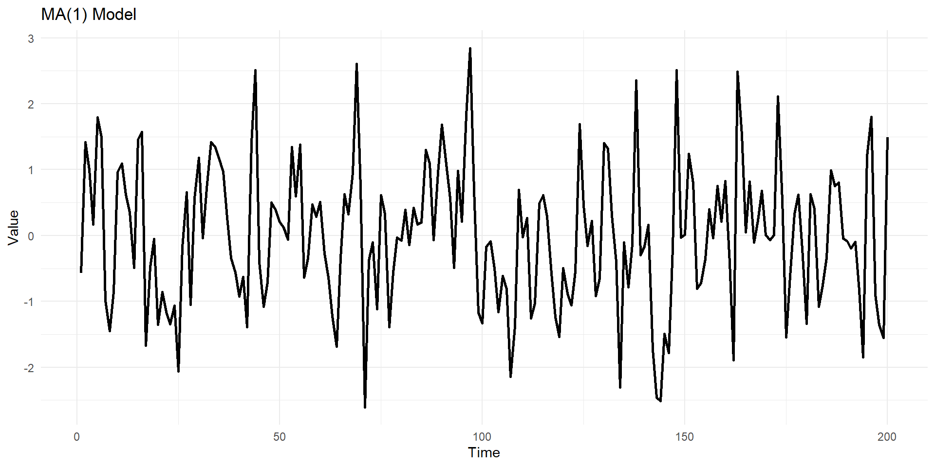
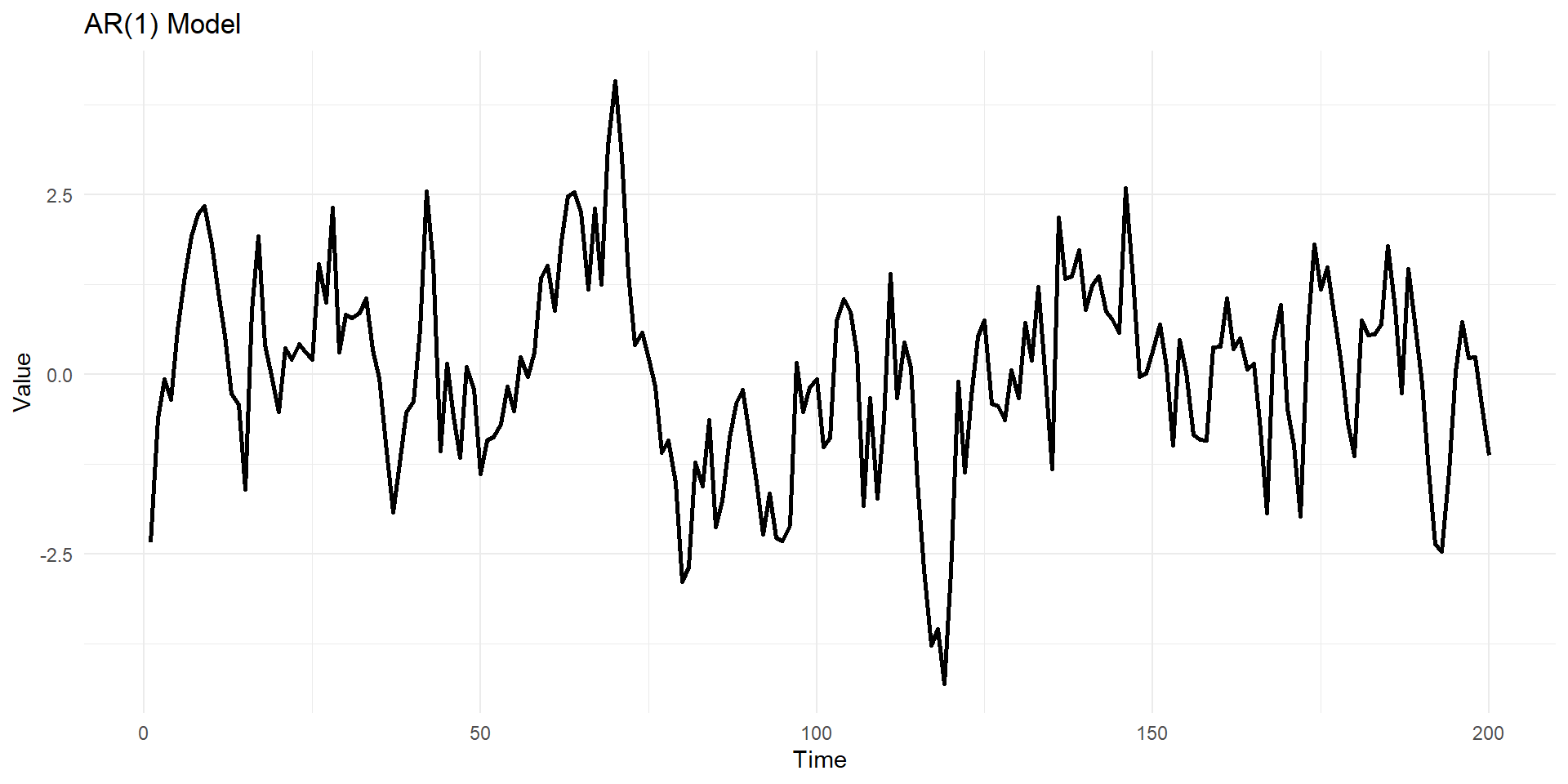
phi <- 0.8  # Autoregressive coefficient
n <- 200    # Number of time points

# Simulate data from the AR(1) model
set.seed(123)  # For reproducibility
ar1_data <- arima.sim(model = list(ar = phi), n = n)
# Create a data frame with time series data
time_series_data <- data.frame(Time = 1:n, Value = ar1_data)
# Create a ggplot2 line plot
ggplot(time_series_data, aes(x = Time, y = Value)) +
  geom_line(linewidth=1) +labs(title = "AR(1) Model ", x = "Time", y = "Value") +
  theme_minimal()
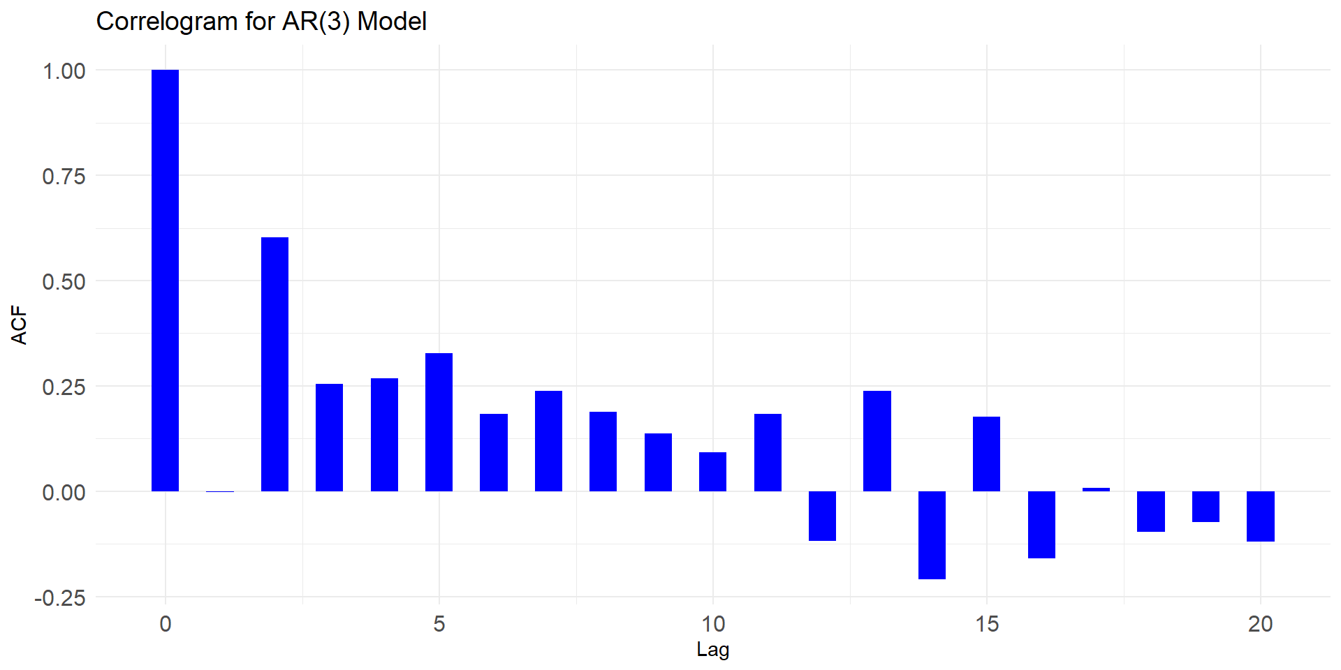
ACF and PACF of AR-1 and MA-`
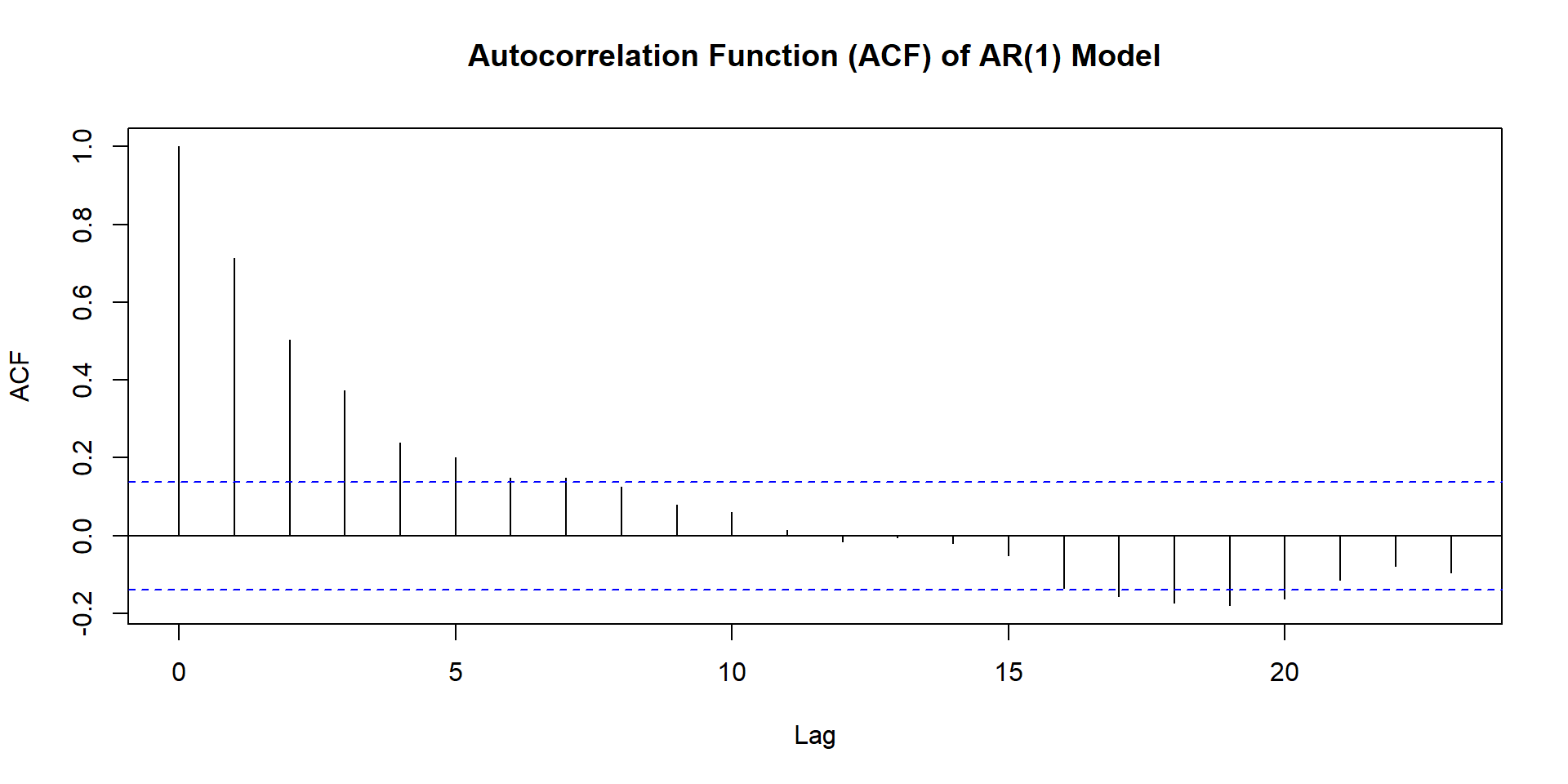
NULL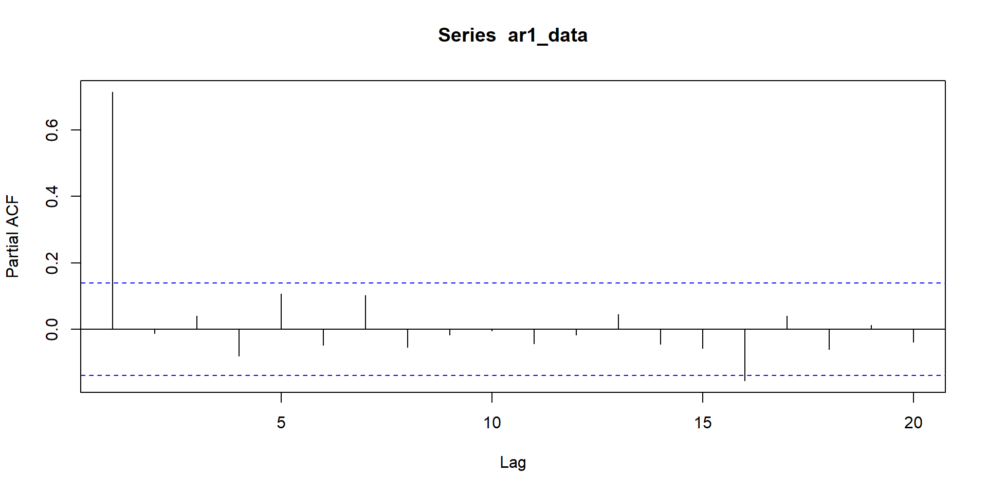
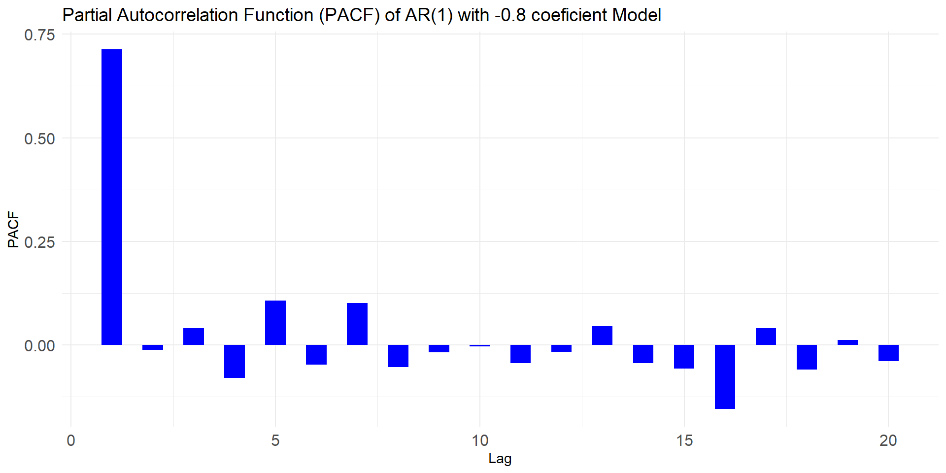
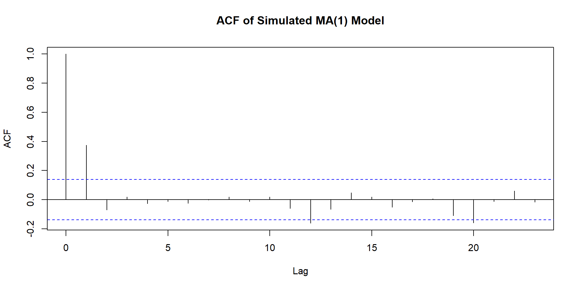
NULL
Now let’s work with real world data
Rows: 733
Columns: 8
$ dateid01 <date> 1954-02-01, 1954-03-01, 1954-04-01, 1954-05-01, 1954-06-01, …
$ dateid   <dttm> 1954-02-28 23:59:59, 1954-03-31 23:59:59, 1954-04-30 23:59:5…
$ date     <date> 1954-02-26, 1954-03-31, 1954-04-30, 1954-05-31, 1954-06-30, …
$ pe_aus   <dbl> NA, NA, NA, NA, NA, NA, NA, NA, NA, NA, NA, NA, NA, NA, NA, N…
$ pe_ind   <dbl> NA, NA, NA, NA, NA, NA, NA, NA, NA, NA, NA, NA, NA, NA, NA, N…
$ pe_ndo   <dbl> NA, NA, NA, NA, NA, NA, NA, NA, NA, NA, NA, NA, NA, NA, NA, N…
$ pe_saf   <dbl> NA, NA, NA, NA, NA, NA, NA, NA, NA, NA, NA, NA, NA, NA, NA, N…
$ pe_usa   <dbl> 9.9200, 10.1700, 10.5700, 11.0000, 11.0800, 12.1740, 11.7600,…
Pick pe_usa
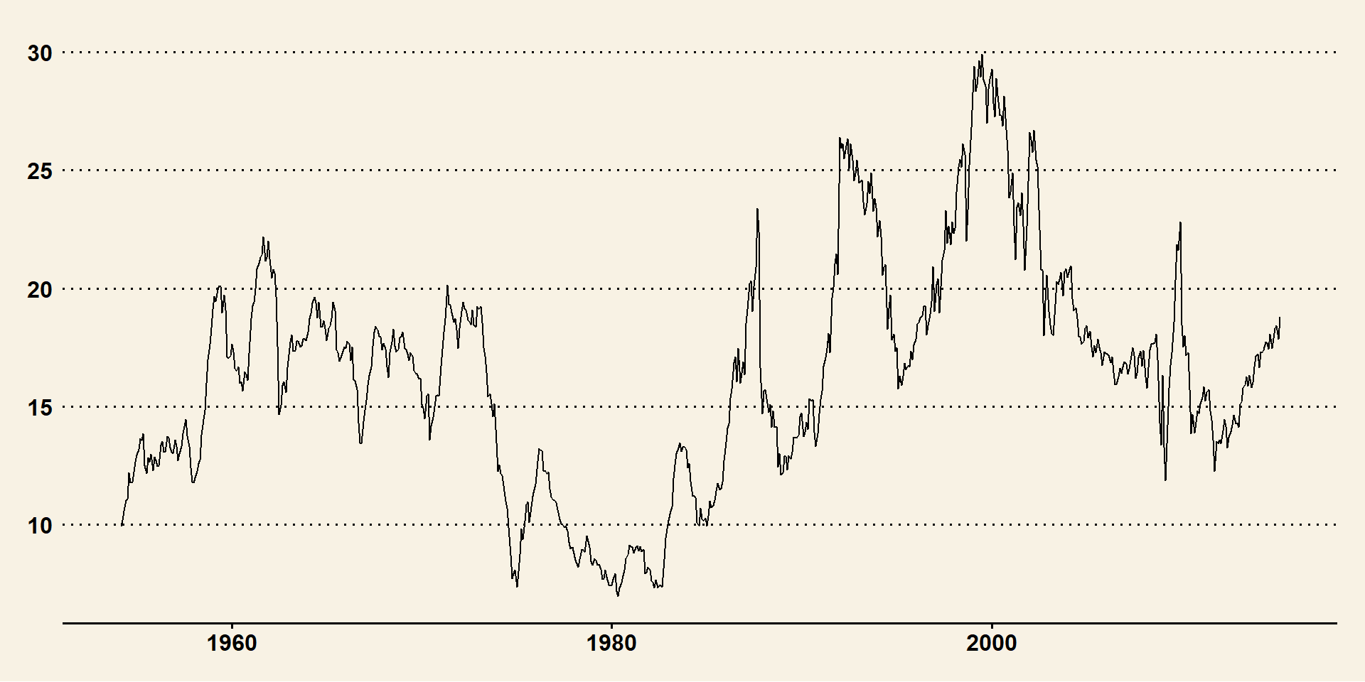
Identify model
Use SACF and SPACF to choose model(s) and also use auto.arima and see which of these two wins: your judged model or auto.arima
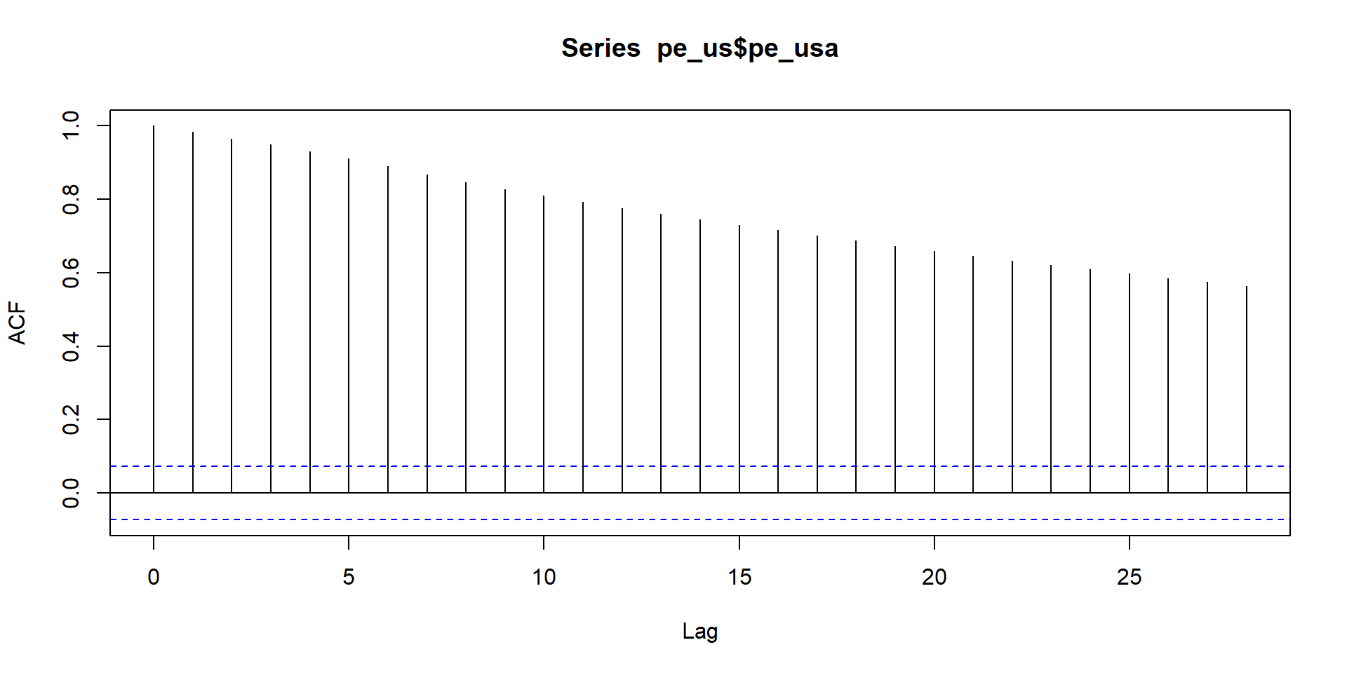
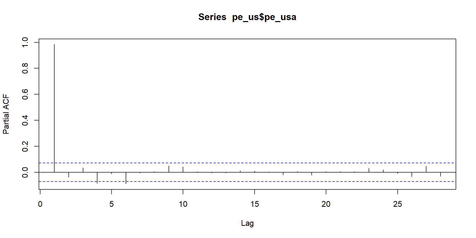
acf and pacf patterns indicate series is non-stationary. So here we run acf and pacf of difference of the series.


From these two graphs it seems model is ARIMA(0,1,1)
Series: pe_us$pe_usa
ARIMA(1,1,1)

Coefficients:
          ar1     ma1
      -0.7554  0.8268
s.e.   0.1106  0.0944

sigma^2 = 0.7151:  log likelihood = -914.95
AIC=1835.91   AICc=1835.94   BIC=1849.69
So our model was ARIMA(0,1,1) while auto.ARIMA is ARIMA(1,1,1) not bad.
Nonstationary Series
Nonstationary Series
- Introduction:
- Key Questions:
- What is nonstationarity?
- Why is it important?
- How do we determine whether a time series is nonstationary?
What is nonstationarity?
Recall from earlier part on stationarity:
- Covariance stationarity of y implies that, over time, y has:
- Constant mean
- Constant variance
- Co-variance between different observations that do not depend on that time (t), only on the “distance” or “lag” between them (j):
\(Cov(Y_t,Y_{tj})= Cov(Y_s,Y_{s+j})= \gamma_j\)
What is nonstatinarity?
Thus, if any of these conditions does not hold, we say that y is nonstationary:
There is no long-run mean to which the series returns (economic concept of long-term equilibrium)
The variance is time-dependent. For example, could go to infinity as the number of observations goes to infinity
Theoretical autocorrelations do not decay, sample autocorrelations do so very slowly.
Nonstationary series can have a trend:
- Deterministic: nonrandom function of time:
\(y_t=\mu+\beta t+u_t\) , where \(u_t\) is “iid”
- Example \(\beta=0.45\)
