Structural VAR Part 1

Zahid Asghar, Professor, School of Economics, QAU

03-12-2023

Introduction

Del Negro and Schorfheide (2011):

At first glance, VARs appear to be straightforward multivariate generalizations of univariate autoregressive models. At second sight, they turn out to be one of the key empirical tools in modern macroeconomics.

What are VARs ?

multivariate linear time-series models
endogenous variable in the system are functions of lagged values of all endogenous variables
simple and flexible alternative to the traditional multiple-equations models

Historical Overview : Sims’ Critique

In the 1980s criticized the large-scale macro-econometric models of the time
Proposed VARs as an alternative that allowed one to model macroeconomic data informatively

What Are VARs Used For?

Forecasting

Reduced Form VARs

Strucutural Analysis

Structural VARs

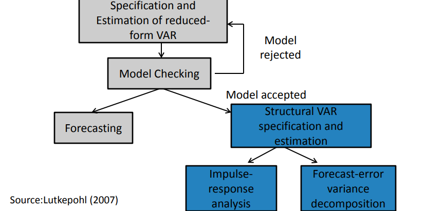
Unit Plan/Roadmap

VAR models roadmap

Estimation of VARs

Introduction to VARs

Let $y_t$ be a vector with the value of $n$ variables at time t:

$y_t=[y_{1,t} y_{2,t} . . . y_{n,t}]'$

A p-order vector autoregressive process generalize a one-variable AR(p) process to n variables:

$y_t=G_0+G_1y_{t-1}+G_2y_{t-2}+...+G_py{t-p}+e_t$ Reduced Form VAR

$G_0=(n.1)$ vector of constraints $G_0=(n.n)$ vector of coefficients $e_t=(n.1)$ vector of white noise innovations

$E[e_t]=0$

$E[e_t e_{\tau}'= \Omega , if t=\tau \\ 0 otherwise$

Example : A VAR(1) in 2 Variables

$y_{1,t}=g_{11}y_{1,t}+g_{12}y_{2,t}+e_{1,t}$

$y_{2,t}=g_{21}y_{1,t}+g_{22}y_{2,t}+e_{2,t}$

$y_t=G_ty_{t-1}+e_t$ where \[y_t=\begin{bmatrix} y_{1,t} \\ y_{2,t} \end{bmatrix}\] \[y_t=\begin{bmatrix} \pi_t \\ gdp_t \end{bmatrix}\]

\[G_t=\begin{bmatrix} g11 & g12 \\ g21 & g22 \\ \end{bmatrix}\]

\[G_t=\begin{bmatrix} e_{1,t} \\ e_{2,t} \end{bmatrix}\], Assumptions about the error terms: \[E[e_te_t']=\begin{bmatrix} 0 & 0\\ 0 & 0 \\ \end{bmatrix}=\Omega, for t\neq\tau\] \[E[e_te_t']=\begin{bmatrix} \sigma_{e1}^2 & \sigma_{e1e2}\\ \sigma_{e1e2} & \sigma_{e2}^2 \\ \end{bmatrix}=\Omega\]

Estimation: by OLS

Performed with OLS applied equation by equation
Estimates are:
- consistent
- efficient
- equivalent to GLS

General Specifications Choices

Selection of variables to be included: in accordance with economic theory, empirical evidence and/or experience
Exogenous variables can be included: constant, time trends, other additional explanators
Non-stationary level data is often transformed (log levels, log differences, growth rates, etc.)
The model should be parsimonious

Stationary VARs

Stationarity of a VAR : Definition

A p-th order VAR is said to be covariance-stationary if :

The expected value of $y_t$ does not depend on timed

\[E[Y_t]=E[Y_{t+j}]=\mu=\begin{bmatrix} \mu_1 \\ \mu_2 \\ \dots \\ \mu_n \end{bmatrix}\] 2. The covariance matrix of $y_t$ and $y_{t+j}$ depends on the time lapsed between j and not not the reference period t

\[E[(y_t-\mu)(y_{t+j}-\mu)']=E[(y_s-\mu)(y_{s+j}-\mu)']=\Gamma_j\]

Condions for Sationarity

The conditioins for a VAR to be stationary are similar to the conditions for a univariate AR process to be stationary: $y_t=G_0+G_1y_{t-1}+G_2 y_{t-2}+\dots+G_py_{t-p}+e_t$

$(I_n-G_1L-G_2L^2-\dots-G_pL^p)y_t=G_0+e_t$

$G(L)y_t=G_0+e_t$ For $y_t$ to be stationary, the matrix polynomial in the lag operator $G(L)$ must be invertible.

Conditions for Stationarity

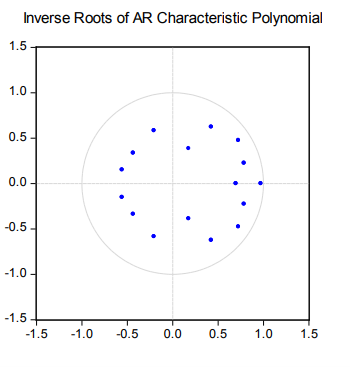
A VAR(p) process is stationary (thus) - A VAR(p) if all the np roots of the characteristic polynomial are (in modulus) outside the unit imaginary

$det(I_n-G_1L-G_2L^2-\dots-G_pL^p)=0$

Softwares sometimes inverse roots of the characteristic AR polynomial, which should then lie within the unit imaginary circle.

Vector Moving Average Representation of a VAR

If a VAR is stationary, the yt vector can be expressed as a sum of all of the past white noise shocks et (VMA(∞) representation $y_t=\mu+G(L)^{-1}e_t$, where $\mu=G(L)^{-1}G_0$ $y_t=\mu+(I_n+\Psi_1L+\Psi L^2+\dots)e_t$ $y_t=\mu+e_t+\Psi e\_{t-1}+\Psi e\_{t-2}+\dots$

$y_t=\mu+\sum_{i=1}^{n} \Psi_i e_{t-i}$

where $\Psi_i$ is a (n x n) matrix of coefficients, and $\Psi_0$ is the identity matrix.
From the VMA($\infty$) representation it is possible to obtain impulse response functions

Lag Specification Criteria

Lags Needed for the VAR

What number is most appropriate? …

If p is extremely short, the model may be poorly specified
If p is extremely long, too many degrees of freedom will be lost
The number of lags should be sufficient for the residuals from the estimation to constitute individual white noises

The Curse of Dimensionality

VARs are very densely parameterized

In a VAR(p) we have p matrices of dimension nxn : $G_1, ...,G_p$
Assume $G_0$ is an intercept vector (dimension: nx1)
The number of total coefficients/parameters to be estimated as : $n+n.n.p=n(1+np)

Overfitting versus Omitted Variable Bias

Over-fitting: poor-quality estimates and bad forecasts
Omitted variable bias: poor-quality estimates and bad forecasts
Possible solutions:
- Core VAR plues rotating variables
- Bayesian Analysis

Lag Selection Criteria

As for univariate models, one can use multidimensional versions of
AIC, BIC, HQ, etc.
Information-based criteria : trade-off between goodness of fit (reduction in Sum of Squares) and parsimony

Lag Specification: Practitioner’s Advice

p=4 when working with quarterly data
p=12 with monthly data
The effective constraint is np<T/3
Example: T=100, $n le 7$, p=4

Forecasting using VARs

Forecasting using the Estimated VAR

Let $Y_{t-1}$ be a matrix containing all information available up to time t (before realization of $e_t$ are known)
Then: $E[y_t/Y_{t-1}]=G_0+G_1y_{t-1}+G_2y_{t-2}+\dots+G_py_{t-p}$

The forecast error can be decomposed into the sum of et , the unexpected innovation of yt , and the coefficient estimation error:

$y_t-E[y_t/Y_{t-1}]=e_t+V(Y_{t-1}])$

If the estimator of the coefficients is consistent and estimates, are based on many data observations, the coefficient estimation error tends to be small, and :

$Y_t-E[y_t/Y_{t-1}]≅e_t$

Iterated Forecasts

Iterating one period forward: $E[y_{t+1}/Y_{t-1}]=G_0+G_1E[y_t|y_{t-1}]+G_2y_{t-2}+\dots+G_py_{t-p+1}$
Iterating j periods forward: $E[y_{t+j}/Y_{t-1}]=G_0+G_1E[y_{t+j-1}|y_{t-1}]+G_2E[y_{t+j-2}|y_{t-1}+\dots+G_py_{t-p+1}$