Bootstrapped Logistic Regression and Machine Learning Models for Predicting Stock Market Movements in the Pakistan Stock Exchange (PSX)

1. Loading and Preparing the Data

The first step is to load the PSX data, clean it, and perform necessary transformations for feature engineering.

library(tidyverse)  # For data manipulation and visualization

Warning: package 'tidyverse' was built under R version 4.5.1

Warning: package 'purrr' was built under R version 4.5.1

── Attaching core tidyverse packages ──────────────────────── tidyverse 2.0.0 ──
✔ dplyr     1.1.4     ✔ readr     2.1.5
✔ forcats   1.0.0     ✔ stringr   1.5.1
✔ ggplot2   3.5.2     ✔ tibble    3.3.0
✔ lubridate 1.9.4     ✔ tidyr     1.3.1
✔ purrr     1.1.0     
── Conflicts ────────────────────────────────────────── tidyverse_conflicts() ──
✖ dplyr::filter() masks stats::filter()
✖ dplyr::lag()    masks stats::lag()
ℹ Use the conflicted package (<http://conflicted.r-lib.org/>) to force all conflicts to become errors

library(caret)      # For model evaluation and cross-validation

Loading required package: lattice

Warning: package 'lattice' was built under R version 4.5.1

Attaching package: 'caret'

The following object is masked from 'package:purrr':

    lift

library(rpart)      # For Decision Trees
library(Metrics)    # For additional evaluation metrics

Warning: package 'Metrics' was built under R version 4.5.1

Attaching package: 'Metrics'

The following objects are masked from 'package:caret':

    precision, recall

library(janitor)    # For cleaning column names

Attaching package: 'janitor'

The following objects are masked from 'package:stats':

    chisq.test, fisher.test

library(MASS)

Attaching package: 'MASS'

The following object is masked from 'package:dplyr':

    select

library(class)    # For KNN
library(boot)

Warning: package 'boot' was built under R version 4.5.1

Attaching package: 'boot'

The following object is masked from 'package:lattice':

    melanoma

We have psx data in csv format. We will load the data and inspect its structure.

psx <- read_csv("data/psx.csv")

Rows: 1827 Columns: 7
── Column specification ────────────────────────────────────────────────────────
Delimiter: ","
chr (3): Date, Vol., Change %
dbl (4): Price, Open, High, Low

ℹ Use `spec()` to retrieve the full column specification for this data.
ℹ Specify the column types or set `show_col_types = FALSE` to quiet this message.

# Inspect the data structure (rows, columns, and types)
dim(psx)

[1] 1827    7

glimpse(psx)

Rows: 1,827
Columns: 7
$ Date       <chr> "11/15/2024", "11/14/2024", "11/13/2024", "11/12/2024", "11…
$ Price      <dbl> 17.42, 17.19, 16.78, 16.86, 17.02, 17.22, 17.14, 17.31, 16.…
$ Open       <dbl> 17.40, 16.70, 16.95, 17.00, 17.46, 17.14, 17.24, 17.24, 17.…
$ High       <dbl> 17.60, 17.60, 16.95, 17.20, 17.46, 17.49, 17.60, 17.50, 17.…
$ Low        <dbl> 16.90, 16.55, 16.50, 16.70, 16.97, 17.01, 17.00, 16.60, 16.…
$ Vol.       <chr> "896.83K", "1.01M", "239.44K", "179.95K", "364.92K", "208.0…
$ `Change %` <chr> "1.34%", "2.44%", "-0.47%", "-0.94%", "-1.16%", "0.47%", "-…

1. Bootstrap Logistic Regression

Apply bootstrap resampling to estimate logistic regression coefficients and evaluate variability.

## Data cleaning and feature engineering


#| label: data-cleaning

# Convert the `Date` column to a proper Date format
psx <- psx %>% 
  mutate(date = as.Date(Date, format = "%m/%d/%Y")) |> dplyr::select(-Date)
# Clean column names to make them consistent and readable
psx <- psx %>% clean_names()

# Convert `change_percent` to numeric and create a new column `direction` for the stock movement (Up/Down)
psx <- psx %>% 
  mutate(
    change_percent = as.numeric(str_remove(change_percent, "%")),
    direction = if_else(change_percent > 0, "Up", "Down")
  )

# Arrange data by ascending date to maintain temporal order
psx <- psx %>% arrange(date)

# Create lag variables for `change_percent` (lags of 1 to 5 days)
psx <- psx %>% 
  mutate(
    lag1 = lag(change_percent, 1),
    lag2 = lag(change_percent, 2),
    lag3 = lag(change_percent, 3),
    lag4 = lag(change_percent, 4),
    lag5 = lag(change_percent, 5)
  )

# Convert `vol` (volume) to numeric, handling the M and K suffixes
psx <- psx %>% mutate(vol = as.numeric(str_replace_all(vol, c("M" = "e6", "K" = "e3"))))

# Drop rows with missing values (NA)
psx_clean <- psx %>% drop_na()

# Convert `direction` to numeric for binary classification (1 for "Up", 0 for "Down")
psx_clean <- psx_clean %>%
  mutate(direction = if_else(direction == "Up", 1, 0))

Define a Bootstrap Function:

boot_logistic <- function(data, indices) {
  sampled_data <- data[indices, ]
  model <- glm(direction ~ lag1 + lag2 + lag3 + lag4 + lag5 + vol, 
               data = sampled_data, family = binomial)
  return(coef(model))
}

Apply Bootstrapping:

set.seed(123)
logistic_boot_result <- boot(data = psx_clean, statistic = boot_logistic, R = 1000)
print(logistic_boot_result)

ORDINARY NONPARAMETRIC BOOTSTRAP


Call:
boot(data = psx_clean, statistic = boot_logistic, R = 1000)


Bootstrap Statistics :
         original        bias     std. error
t1* -5.236745e-01 -2.097142e-03 6.719302e-02
t2* -6.414172e-02  7.111280e-05 1.749324e-02
t3* -1.149754e-02  1.149087e-04 1.588335e-02
t4* -4.222881e-03  7.199437e-04 1.633129e-02
t5* -2.171095e-02 -1.378824e-03 1.638450e-02
t6* -4.423349e-02 -1.337178e-03 1.472036e-02
t7*  4.183911e-07  4.427846e-09 5.749570e-08

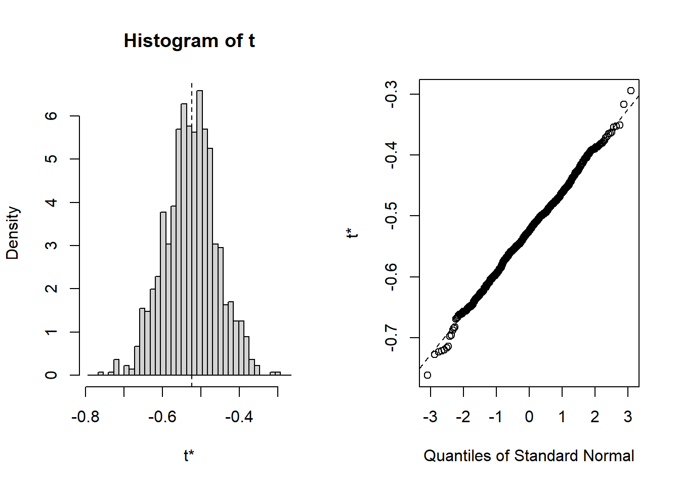
Visualize and Extract Confidence Intervals:

plot(logistic_boot_result)

boot.ci(boot.out = logistic_boot_result, type = c("norm", "basic", "perc"))

BOOTSTRAP CONFIDENCE INTERVAL CALCULATIONS
Based on 1000 bootstrap replicates

CALL : 
boot.ci(boot.out = logistic_boot_result, type = c("norm", "basic", 
    "perc"))

Intervals : 
Level      Normal              Basic              Percentile     
95%   (-0.6533, -0.3899 )   (-0.6570, -0.3905 )   (-0.6568, -0.3903 )  
Calculations and Intervals on Original Scale

---

2. Bootstrap for LDA

Define a Bootstrap Function:

boot_lda <- function(data, indices) {
  sampled_data <- data[indices, ]
  lda_model <- lda(direction ~ lag1 + lag2 + lag3 + lag4 + lag5 + vol, 
                    data = sampled_data)
  predictions <- predict(lda_model, newdata = data)$class
  accuracy <- mean(predictions == data$direction)
  return(accuracy)
}

Apply Bootstrapping:

set.seed(123)
lda_boot_result <- boot(data = psx_clean, statistic = boot_lda, R = 500)
print(lda_boot_result)

ORDINARY NONPARAMETRIC BOOTSTRAP


Call:
boot(data = psx_clean, statistic = boot_lda, R = 500)


Bootstrap Statistics :
     original     bias    std. error
t1* 0.6053787 0.00270472 0.004244633

---

3. Bootstrap for QDA

Define a Bootstrap Function:

boot_qda <- function(data, indices) {
  sampled_data <- data[indices, ]
  qda_model <- qda(direction ~ lag1 + lag2 + lag3 + lag4 + lag5 + vol, 
                    data = sampled_data)
  predictions <- predict(qda_model, newdata = data)$class
  accuracy <- mean(predictions == data$direction)
  return(accuracy)
}

Apply Bootstrapping:

set.seed(123)
qda_boot_result <- boot(data = psx_clean, statistic = boot_qda, R = 500)
print(qda_boot_result)

ORDINARY NONPARAMETRIC BOOTSTRAP


Call:
boot(data = psx_clean, statistic = boot_qda, R = 500)


Bootstrap Statistics :
     original       bias    std. error
t1* 0.5944018 -0.003982437  0.01522457

---

4. Bootstrap for KNN

Define a Bootstrap Function:

boot_knn <- function(data, indices) {
  train_data <- data[indices, ]
  test_data <- data[-indices, ]
  knn_model <- knn(
    train = train_data[, c("lag1", "lag2", "lag3", "lag4", "lag5", "vol")],
    test = test_data[, c("lag1", "lag2", "lag3", "lag4", "lag5", "vol")],
    cl = train_data$direction,
    k = 5
  )
  accuracy <- mean(knn_model == test_data$direction)
  return(accuracy)
}

Apply Bootstrapping:

set.seed(123)
knn_boot_result <- boot(data = psx_clean, statistic = boot_knn, R = 500)
print(knn_boot_result)

ORDINARY NONPARAMETRIC BOOTSTRAP


Call:
boot(data = psx_clean, statistic = boot_knn, R = 500)


Bootstrap Statistics :
    original  bias    std. error
t1*      NaN     NaN  0.01808283

---

5. Bootstrap for Decision Trees

Define a Bootstrap Function:

boot_dt <- function(data, indices) {
  sampled_data <- data[indices, ]
  tree_model <- rpart(direction ~ lag1 + lag2 + lag3 + lag4 + lag5 + vol, 
                      data = sampled_data, method = "class")
  predictions <- predict(tree_model, newdata = data, type = "class")
  accuracy <- mean(predictions == data$direction)
  return(accuracy)
}

Apply Bootstrapping:

set.seed(123)
dt_boot_result <- boot(data = psx_clean, statistic = boot_dt, R = 500)
print(dt_boot_result)

ORDINARY NONPARAMETRIC BOOTSTRAP


Call:
boot(data = psx_clean, statistic = boot_dt, R = 500)


Bootstrap Statistics :
     original        bias    std. error
t1* 0.6262349 -0.0005060373   0.0107856

---

Summarize Results:

Aggregate accuracy or coefficients across models to compare:

list(
  logistic = mean(logistic_boot_result$t),
  lda = mean(lda_boot_result$t),
  qda = mean(qda_boot_result$t),
  knn = mean(knn_boot_result$t),
  decision_tree = mean(dt_boot_result$t)
)

$logistic
[1] -0.09619826

$lda
[1] 0.6080834

$qda
[1] 0.5904193

$knn
[1] 0.5456178

$decision_tree
[1] 0.6257289