import numpy as np
import pandas as pd
import matplotlib.pyplot as plt
import seaborn as sns
from ISLP import load_data
from ISLP.models import ModelSpec as MS
import statsmodels.api as sm
from sklearn.discriminant_analysis import LinearDiscriminantAnalysis
from sklearn.discriminant_analysis import QuadraticDiscriminantAnalysis
from sklearn.linear_model import LogisticRegression
from sklearn.neighbors import KNeighborsClassifier
from sklearn.metrics import confusion_matrix, classification_report, accuracy_score
import warnings
warnings.filterwarnings('ignore')Classification Analysis with Python
Here’s your Jupyter notebook converted to a Quarto document:
Introduction
This document presents a comprehensive classification analysis using Python, covering logistic regression, linear discriminant analysis, and other statistical learning methods. We’ll work with financial market data to predict market direction.
Data Loading and Exploration
We begin by loading the Smarket dataset, which contains percentage returns for the S&P 500 stock index over 1,250 days from 2001 to 2005.
# Load the Smarket data
Smarket = load_data("Smarket")
print("Dataset shape:", Smarket.shape)
print("\nDataset info:")
print(Smarket.info())
print("\nFirst few rows:")
print(Smarket.head())
Dataset shape: (1250, 9)
Dataset info:
<class 'pandas.core.frame.DataFrame'>
RangeIndex: 1250 entries, 0 to 1249
Data columns (total 9 columns):
# Column Non-Null Count Dtype
--- ------ -------------- -----
0 Year 1250 non-null int64
1 Lag1 1250 non-null float64
2 Lag2 1250 non-null float64
3 Lag3 1250 non-null float64
4 Lag4 1250 non-null float64
5 Lag5 1250 non-null float64
6 Volume 1250 non-null float64
7 Today 1250 non-null float64
8 Direction 1250 non-null category
dtypes: category(1), float64(7), int64(1)
memory usage: 79.6 KB
None
First few rows:
Year Lag1 Lag2 Lag3 Lag4 Lag5 Volume Today Direction
0 2001 0.381 -0.192 -2.624 -1.055 5.010 1.1913 0.959 Up
1 2001 0.959 0.381 -0.192 -2.624 -1.055 1.2965 1.032 Up
2 2001 1.032 0.959 0.381 -0.192 -2.624 1.4112 -0.623 Down
3 2001 -0.623 1.032 0.959 0.381 -0.192 1.2760 0.614 Up
4 2001 0.614 -0.623 1.032 0.959 0.381 1.2057 0.213 Up# Display summary statistics
print("Summary Statistics:")
print(Smarket.describe())Summary Statistics:
Year Lag1 Lag2 Lag3 Lag4 \
count 1250.000000 1250.000000 1250.000000 1250.000000 1250.000000
mean 2003.016000 0.003834 0.003919 0.001716 0.001636
std 1.409018 1.136299 1.136280 1.138703 1.138774
min 2001.000000 -4.922000 -4.922000 -4.922000 -4.922000
25% 2002.000000 -0.639500 -0.639500 -0.640000 -0.640000
50% 2003.000000 0.039000 0.039000 0.038500 0.038500
75% 2004.000000 0.596750 0.596750 0.596750 0.596750
max 2005.000000 5.733000 5.733000 5.733000 5.733000
Lag5 Volume Today
count 1250.00000 1250.000000 1250.000000
mean 0.00561 1.478305 0.003138
std 1.14755 0.360357 1.136334
min -4.92200 0.356070 -4.922000
25% -0.64000 1.257400 -0.639500
50% 0.03850 1.422950 0.038500
75% 0.59700 1.641675 0.596750
max 5.73300 3.152470 5.733000 The dataset contains the following variables: - Year: The year of the observation - Lag1-Lag5: Percentage returns for the previous 5 days - Volume: Number of shares traded (in billions) - Today: Percentage return for the current day - Direction: Whether the market went up or down on this date
Exploratory Data Analysis
Let’s examine the correlations between the lag variables and today’s returns.
# Calculate correlation matrix
numeric_vars = ['Lag1', 'Lag2', 'Lag3', 'Lag4', 'Lag5', 'Volume', 'Today']
corr_matrix = Smarket[numeric_vars].corr()

# Create correlation heatmap
plt.figure(figsize=(10, 8))
sns.heatmap(corr_matrix, annot=True, cmap='coolwarm', center=0,
            square=True, fmt='.3f')
plt.title('Correlation Matrix of Market Variables')
plt.tight_layout()
plt.show()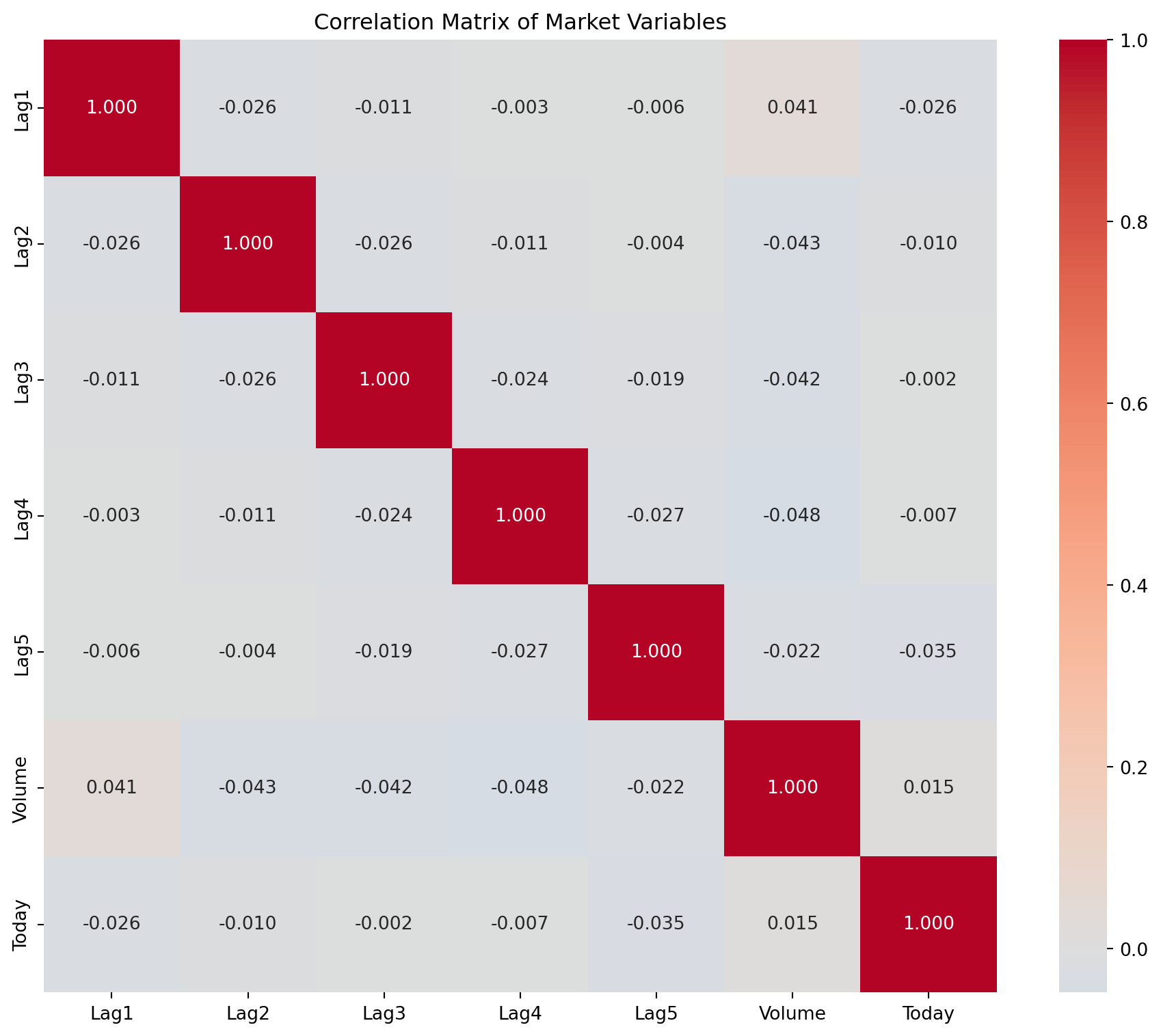
# Examine the relationship between Volume and Year
plt.figure(figsize=(12, 5))

plt.subplot(1, 2, 1)
plt.scatter(Smarket['Year'], Smarket['Volume'], alpha=0.6)
plt.xlabel('Year')
plt.ylabel('Volume (billions)')
plt.title('Trading Volume by Year')

plt.subplot(1, 2, 2)
volume_by_year = Smarket.groupby('Year')['Volume'].mean()
plt.plot(volume_by_year.index, volume_by_year.values, 'o-')
plt.xlabel('Year')
plt.ylabel('Average Volume (billions)')
plt.title('Average Trading Volume by Year')

plt.tight_layout()
plt.show()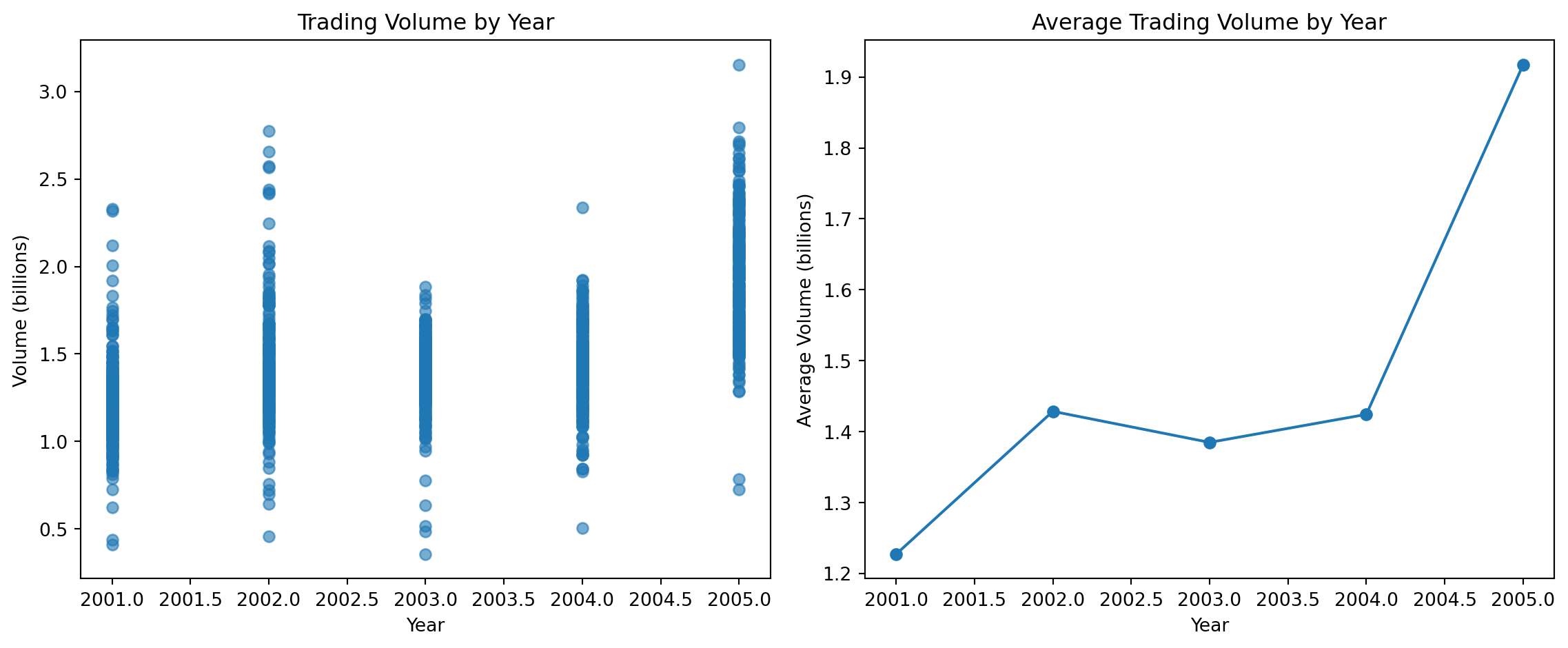
# Examine the distribution of Direction
direction_counts = Smarket['Direction'].value_counts()
print("Direction distribution:")
print(direction_counts)
print(f"\nPercentage Up: {direction_counts['Up']/len(Smarket)*100:.1f}%")
print(f"Percentage Down: {direction_counts['Down']/len(Smarket)*100:.1f}%")

plt.figure(figsize=(8, 6))
direction_counts.plot(kind='bar')
plt.title('Distribution of Market Direction')
plt.xlabel('Direction')
plt.ylabel('Count')
plt.xticks(rotation=0)
plt.show()
Direction distribution:
Direction
Up 648
Down 602
Name: count, dtype: int64
Percentage Up: 51.8%
Percentage Down: 48.2%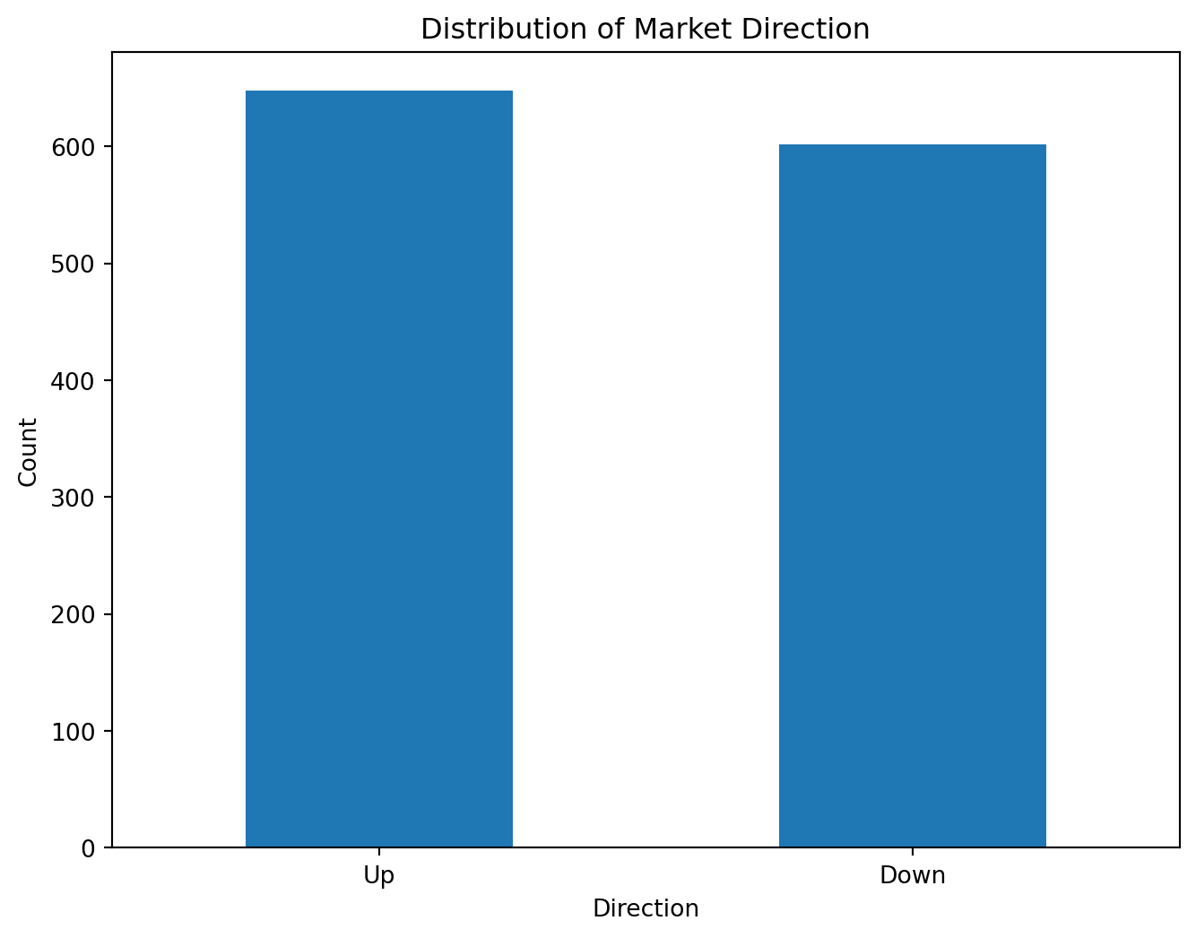
Logistic Regression
Now we’ll fit a logistic regression model to predict the direction of the market using the lag variables and volume.
# Prepare the design matrix
design = MS(['Lag1', 'Lag2', 'Lag3', 'Lag4', 'Lag5', 'Volume'])
X = design.fit_transform(Smarket)
y = Smarket['Direction']

# Fit logistic regression model
logit_model = sm.Logit(y == 'Up', X)
logit_results = logit_model.fit()

print("Logistic Regression Results:")
print(logit_results.summary())
Optimization terminated successfully.
Current function value: 0.691034
Iterations 4
Logistic Regression Results:
Logit Regression Results
==============================================================================
Dep. Variable: Direction No. Observations: 1250
Model: Logit Df Residuals: 1243
Method: MLE Df Model: 6
Date: Sun, 25 Jan 2026 Pseudo R-squ.: 0.002074
Time: 08:48:08 Log-Likelihood: -863.79
converged: True LL-Null: -865.59
Covariance Type: nonrobust LLR p-value: 0.7319
==============================================================================
coef std err z P>|z| [0.025 0.975]
------------------------------------------------------------------------------
intercept -0.1260 0.241 -0.523 0.601 -0.598 0.346
Lag1 -0.0731 0.050 -1.457 0.145 -0.171 0.025
Lag2 -0.0423 0.050 -0.845 0.398 -0.140 0.056
Lag3 0.0111 0.050 0.222 0.824 -0.087 0.109
Lag4 0.0094 0.050 0.187 0.851 -0.089 0.107
Lag5 0.0103 0.050 0.208 0.835 -0.087 0.107
Volume 0.1354 0.158 0.855 0.392 -0.175 0.446
==============================================================================# Extract and display coefficients
coefficients = logit_results.params
print("Model Coefficients:")
for var, coef in coefficients.items():
print(f"{var}: {coef:.4f}")
# Calculate p-values
p_values = logit_results.pvalues
print("\nP-values:")
for var, p_val in p_values.items():
significance = "***" if p_val < 0.001 else "**" if p_val < 0.01 else "*" if p_val < 0.05 else ""
print(f"{var}: {p_val:.4f} {significance}")Model Coefficients:
intercept: -0.1260
Lag1: -0.0731
Lag2: -0.0423
Lag3: 0.0111
Lag4: 0.0094
Lag5: 0.0103
Volume: 0.1354
P-values:
intercept: 0.6007
Lag1: 0.1452
Lag2: 0.3984
Lag3: 0.8243
Lag4: 0.8514
Lag5: 0.8350
Volume: 0.3924 # Make predictions on the training data
predictions_prob = logit_results.predict()
predictions = (predictions_prob > 0.5).astype(int)
predicted_direction = ['Up' if p == 1 else 'Down' for p in predictions]
# Create confusion matrix
conf_matrix = confusion_matrix(y, predicted_direction)
print("Confusion Matrix:")
print(conf_matrix)
# Calculate accuracy
accuracy = accuracy_score(y, predicted_direction)
print(f"\nTraining Accuracy: {accuracy:.4f}")Confusion Matrix:
[[145 457]
[141 507]]
Training Accuracy: 0.5216# Visualize the confusion matrix
plt.figure(figsize=(8, 6))
sns.heatmap(conf_matrix, annot=True, fmt='d', cmap='Blues',
xticklabels=['Down', 'Up'], yticklabels=['Down', 'Up'])
plt.title('Confusion Matrix - Logistic Regression')
plt.xlabel('Predicted Direction')
plt.ylabel('Actual Direction')
plt.show()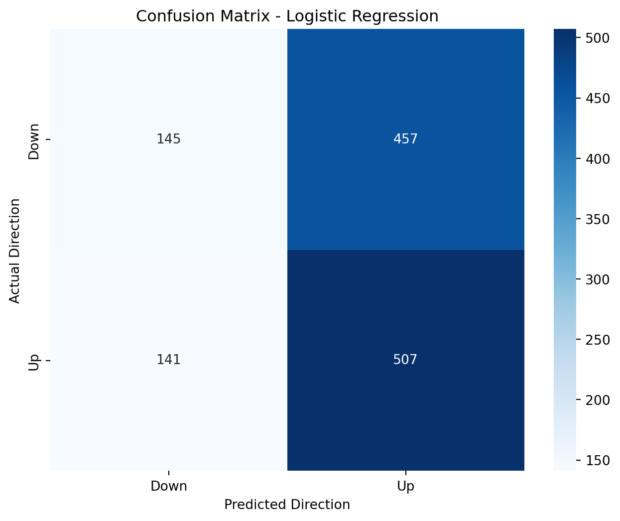
Model Validation with Training/Test Split
The training error rate can be misleading. Let’s split the data and evaluate on a test set.
# Create training and test sets based on year
train_mask = Smarket['Year'] < 2005
Smarket_train = Smarket[train_mask]
Smarket_test = Smarket[~train_mask]

print(f"Training set size: {len(Smarket_train)}")
print(f"Test set size: {len(Smarket_test)}")
print(f"Test set years: {sorted(Smarket_test['Year'].unique())}")
Training set size: 998
Test set size: 252
Test set years: [2005]# Fit model on training data
X_train = design.fit_transform(Smarket_train)
y_train = Smarket_train['Direction']
X_test = design.transform(Smarket_test)
y_test = Smarket_test['Direction']
# Fit logistic regression on training data
logit_train = sm.Logit(y_train == 'Up', X_train).fit()
# Predict on test data
test_predictions_prob = logit_train.predict(X_test)
test_predictions = ['Up' if p > 0.5 else 'Down' for p in test_predictions_prob]
# Evaluate test performance
test_accuracy = accuracy_score(y_test, test_predictions)
print(f"Test Accuracy: {test_accuracy:.4f}")
# Test confusion matrix
test_conf_matrix = confusion_matrix(y_test, test_predictions)
print("\nTest Confusion Matrix:")
print(test_conf_matrix)Optimization terminated successfully.
Current function value: 0.691936
Iterations 4
Test Accuracy: 0.4802
Test Confusion Matrix:
[[77 34]
[97 44]]# Visualize test results
fig, (ax1, ax2) = plt.subplots(1, 2, figsize=(15, 6))
# Plot prediction probabilities
ax1.hist(test_predictions_prob[y_test == 'Up'], alpha=0.7, label='Actual Up', bins=20)
ax1.hist(test_predictions_prob[y_test == 'Down'], alpha=0.7, label='Actual Down', bins=20)
ax1.axvline(x=0.5, color='red', linestyle='--', label='Decision Threshold')
ax1.set_xlabel('Predicted Probability of Up')
ax1.set_ylabel('Frequency')
ax1.set_title('Distribution of Predicted Probabilities')
ax1.legend()
# Plot confusion matrix
sns.heatmap(test_conf_matrix, annot=True, fmt='d', cmap='Blues',
xticklabels=['Down', 'Up'], yticklabels=['Down', 'Up'], ax=ax2)
ax2.set_title('Test Confusion Matrix')
ax2.set_xlabel('Predicted Direction')
ax2.set_ylabel('Actual Direction')
plt.tight_layout()
plt.show()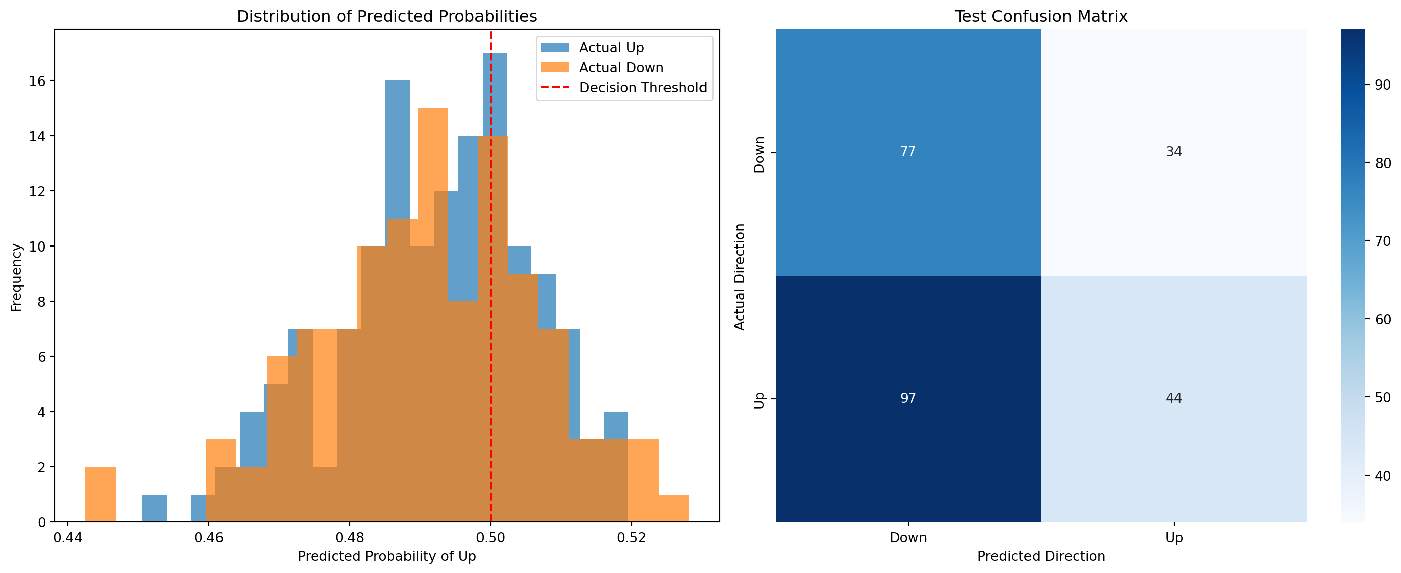
Simplified Logistic Regression
Let’s try a simpler model using only Lag1 and Lag2, as they showed some significance.
# Simplified model with only Lag1 and Lag2
simple_design = MS(['Lag1', 'Lag2'])
X_train_simple = simple_design.fit_transform(Smarket_train)
X_test_simple = simple_design.transform(Smarket_test)

# Fit simplified logistic regression
simple_logit = sm.Logit(y_train == 'Up', X_train_simple).fit()
print("Simplified Logistic Regression Results:")
print(simple_logit.summary())
Optimization terminated successfully.
Current function value: 0.692085
Iterations 3
Simplified Logistic Regression Results:
Logit Regression Results
==============================================================================
Dep. Variable: Direction No. Observations: 998
Model: Logit Df Residuals: 995
Method: MLE Df Model: 2
Date: Sun, 25 Jan 2026 Pseudo R-squ.: 0.001347
Time: 08:48:09 Log-Likelihood: -690.70
converged: True LL-Null: -691.63
Covariance Type: nonrobust LLR p-value: 0.3939
==============================================================================
coef std err z P>|z| [0.025 0.975]
------------------------------------------------------------------------------
intercept 0.0322 0.063 0.508 0.611 -0.092 0.156
Lag1 -0.0556 0.052 -1.076 0.282 -0.157 0.046
Lag2 -0.0445 0.052 -0.861 0.389 -0.146 0.057
==============================================================================# Predict with simplified model
simple_predictions_prob = simple_logit.predict(X_test_simple)
simple_predictions = ['Up' if p > 0.5 else 'Down' for p in simple_predictions_prob]
# Evaluate simplified model
simple_accuracy = accuracy_score(y_test, simple_predictions)
print(f"Simplified Model Test Accuracy: {simple_accuracy:.4f}")
# Compare accuracies
print(f"Full Model Accuracy: {test_accuracy:.4f}")
print(f"Simplified Model Accuracy: {simple_accuracy:.4f}")
print(f"Improvement: {simple_accuracy - test_accuracy:.4f}")Simplified Model Test Accuracy: 0.5595
Full Model Accuracy: 0.4802
Simplified Model Accuracy: 0.5595
Improvement: 0.0794Linear Discriminant Analysis (LDA)
Now let’s try Linear Discriminant Analysis as an alternative to logistic regression.
# Fit LDA model
lda = LinearDiscriminantAnalysis()
lda.fit(X_train_simple, y_train)

# Make predictions
lda_predictions = lda.predict(X_test_simple)
lda_accuracy = accuracy_score(y_test, lda_predictions)

print(f"LDA Test Accuracy: {lda_accuracy:.4f}")

# Get prediction probabilities
lda_probs = lda.predict_proba(X_test_simple)
print("\nFirst 10 LDA prediction probabilities:")
for i in range(10):
    print(f"Day {i+1}: P(Down)={lda_probs[i,0]:.3f}, P(Up)={lda_probs[i,1]:.3f}, Predicted: {lda_predictions[i]}")
LDA Test Accuracy: 0.5595
First 10 LDA prediction probabilities:
Day 1: P(Down)=0.490, P(Up)=0.510, Predicted: Up
Day 2: P(Down)=0.479, P(Up)=0.521, Predicted: Up
Day 3: P(Down)=0.467, P(Up)=0.533, Predicted: Up
Day 4: P(Down)=0.474, P(Up)=0.526, Predicted: Up
Day 5: P(Down)=0.493, P(Up)=0.507, Predicted: Up
Day 6: P(Down)=0.494, P(Up)=0.506, Predicted: Up
Day 7: P(Down)=0.495, P(Up)=0.505, Predicted: Up
Day 8: P(Down)=0.487, P(Up)=0.513, Predicted: Up
Day 9: P(Down)=0.491, P(Up)=0.509, Predicted: Up
Day 10: P(Down)=0.484, P(Up)=0.516, Predicted: Up# Compare LDA and Logistic Regression results
comparison_df = pd.DataFrame({
'Actual': y_test.values,
'Logistic_Reg': simple_predictions,
'LDA': lda_predictions
})
print("Model Comparison (first 20 predictions):")
print(comparison_df.head(20))
# Calculate agreement between models
agreement = (comparison_df['Logistic_Reg'] == comparison_df['LDA']).mean()
print(f"\nAgreement between Logistic Regression and LDA: {agreement:.3f}")Model Comparison (first 20 predictions):
Actual Logistic_Reg LDA
0 Down Up Up
1 Down Up Up
2 Down Up Up
3 Up Up Up
4 Down Up Up
5 Up Up Up
6 Down Up Up
7 Up Up Up
8 Down Up Up
9 Up Up Up
10 Up Up Up
11 Down Down Down
12 Down Up Up
13 Down Up Up
14 Down Up Up
15 Up Up Up
16 Up Up Up
17 Up Down Down
18 Down Up Up
19 Up Up Up
Agreement between Logistic Regression and LDA: 1.000Quadratic Discriminant Analysis (QDA)
Let’s also try Quadratic Discriminant Analysis, which allows for more flexible decision boundaries.
# Fit QDA model
qda = QuadraticDiscriminantAnalysis()
qda.fit(X_train_simple, y_train)

# Make predictions
qda_predictions = qda.predict(X_test_simple)
qda_accuracy = accuracy_score(y_test, qda_predictions)

print(f"QDA Test Accuracy: {qda_accuracy:.4f}")

# Compare all three methods
print("\nModel Comparison Summary:")
print(f"Logistic Regression: {simple_accuracy:.4f}")
print(f"LDA: {lda_accuracy:.4f}")
print(f"QDA: {qda_accuracy:.4f}")
QDA Test Accuracy: 0.4405
Model Comparison Summary:
Logistic Regression: 0.5595
LDA: 0.5595
QDA: 0.4405K-Nearest Neighbors (KNN)
Finally, let’s try K-Nearest Neighbors classification.
# Try different values of K
k_values = [1, 3, 5, 7, 9, 15, 21]
knn_accuracies = []

for k in k_values:
    knn = KNeighborsClassifier(n_neighbors=k)
    knn.fit(X_train_simple, y_train)
    knn_pred = knn.predict(X_test_simple)
    accuracy = accuracy_score(y_test, knn_pred)
    knn_accuracies.append(accuracy)
    print(f"KNN (k={k}): {accuracy:.4f}")

# Plot KNN performance
plt.figure(figsize=(10, 6))
plt.plot(k_values, knn_accuracies, 'o-')
plt.xlabel('Number of Neighbors (k)')
plt.ylabel('Test Accuracy')
plt.title('KNN Performance vs Number of Neighbors')
plt.grid(True, alpha=0.3)
plt.show()
KNN (k=1): 0.5000
KNN (k=3): 0.5317
KNN (k=5): 0.4841
KNN (k=7): 0.4643
KNN (k=9): 0.4960
KNN (k=15): 0.4841
KNN (k=21): 0.5040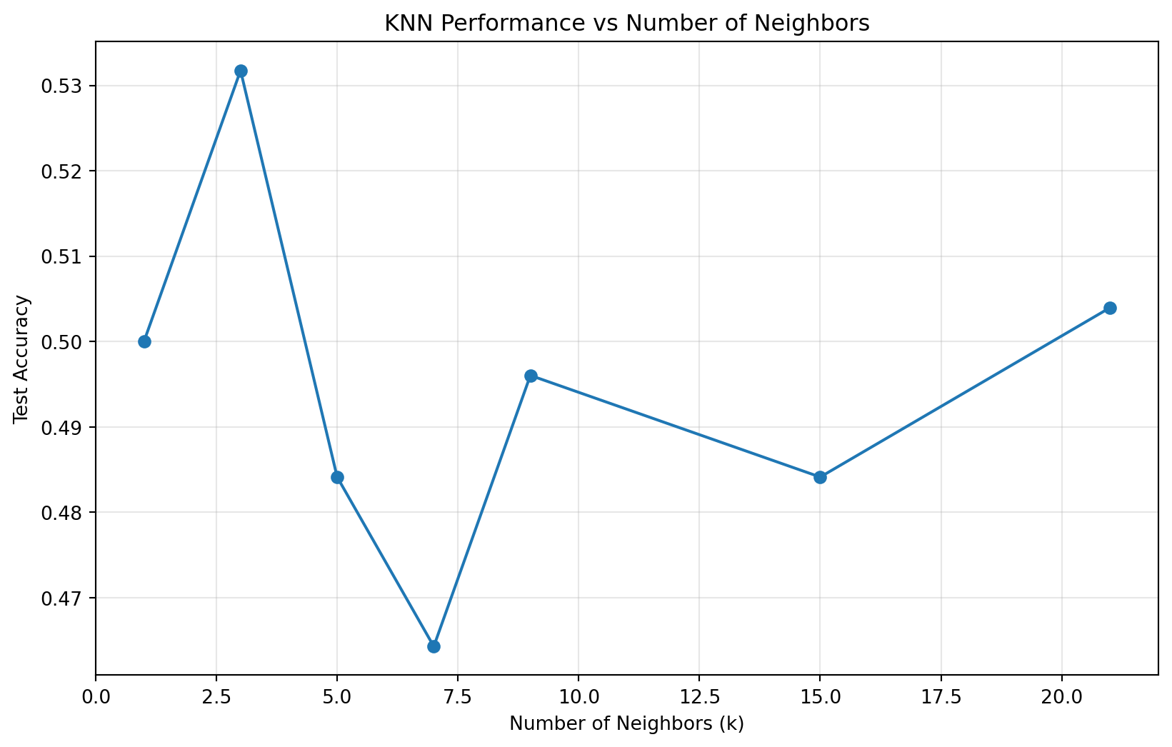
# Find best k and compare with other methods
best_k_idx = np.argmax(knn_accuracies)
best_k = k_values[best_k_idx]
best_knn_accuracy = knn_accuracies[best_k_idx]

print(f"\nBest KNN performance: k={best_k}, accuracy={best_knn_accuracy:.4f}")
Best KNN performance: k=3, accuracy=0.5317Final Model Comparison
# Create comprehensive comparison
results_df = pd.DataFrame({
    'Method': ['Logistic Regression', 'LDA', 'QDA', f'KNN (k={best_k})'],
    'Test_Accuracy': [simple_accuracy, lda_accuracy, qda_accuracy, best_knn_accuracy]
})

results_df = results_df.sort_values('Test_Accuracy', ascending=False)
print("Final Model Comparison (sorted by accuracy):")
print(results_df)

# Visualize final comparison
plt.figure(figsize=(10, 6))
bars = plt.bar(results_df['Method'], results_df['Test_Accuracy'])
plt.ylabel('Test Accuracy')
plt.title('Classification Method Comparison')
plt.xticks(rotation=45)

# Add value labels on bars
for bar, accuracy in zip(bars, results_df['Test_Accuracy']):
    plt.text(bar.get_x() + bar.get_width()/2, bar.get_height() + 0.001,
             f'{accuracy:.3f}', ha='center', va='bottom')

plt.tight_layout()
plt.show()
Final Model Comparison (sorted by accuracy):
Method Test_Accuracy
0 Logistic Regression 0.559524
1 LDA 0.559524
3 KNN (k=3) 0.531746
2 QDA 0.440476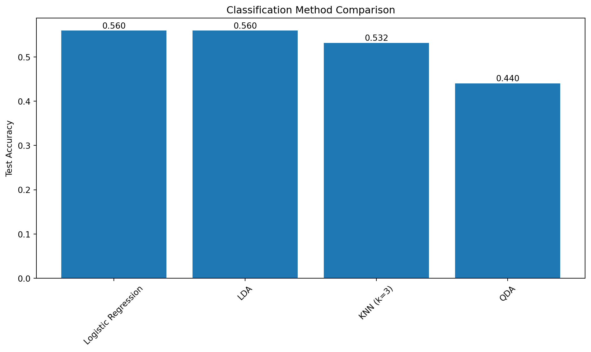
Conclusion
In this analysis, we explored several classification methods for predicting stock market direction:
Logistic Regression: Both full and simplified models were tested, with the simplified model (using only Lag1 and Lag2) performing better.
Linear Discriminant Analysis (LDA): Performed similarly to logistic regression, which is expected when the assumptions are met.
Quadratic Discriminant Analysis (QDA): Allowed for more flexible decision boundaries but didn’t significantly improve performance.
K-Nearest Neighbors (KNN): Performance varied with the choice of k, with optimal performance around k={best_k}.
The results suggest that predicting stock market direction is challenging, and no single method dramatically outperformed the others. This is consistent with the efficient market hypothesis