Step-by-Step Guide in R:

1. Understanding Bootstrapping

Bootstrapping is a resampling method that involves randomly drawing samples from a dataset with replacement. It is commonly used to estimate the variability of a statistic (e.g., mean, median, regression coefficient).

2. Setup

Install and load the necessary libraries:

#install.packages("ISLR")  # Contains datasets used in "Introduction to Statistical Learning"
#install.packages("boot")  # Bootstrapping functions
library(ISLR2)
library(boot)

3. Select a Dataset

Use the Auto dataset from the ISLR package as an example:

data("Auto")

4. Define a Statistic

Choose a statistic to compute. For example, estimating the mean of mpg:

mean_mpg <- function(data, indices) {
  sampled_data <- data[indices]  # Resample using indices
  return(mean(sampled_data))
}

5. Apply the Bootstrapping

Use the boot function to perform bootstrapping:

set.seed(123)  # For reproducibility
boot_result <- boot(data = Auto$mpg, statistic = mean_mpg, R = 1000)  # 1000 bootstrap samples

6. View the Results

Print the bootstrap estimate and plot:

mean(Auto$mpg)  # Original mean

[1] 23.44592

print(boot_result)

ORDINARY NONPARAMETRIC BOOTSTRAP


Call:
boot(data = Auto$mpg, statistic = mean_mpg, R = 1000)


Bootstrap Statistics :
    original       bias    std. error
t1* 23.44592 -0.008097704   0.4007151

#sample(Auto$mpg, 10, replace = TRUE)  # Example of resampling (with replacement)
# Pairwise sample of mpg and horsepower

#sample(c(Auto$mpg,Auto$horsepower) , 10, replace = TRUE)


plot(boot_result)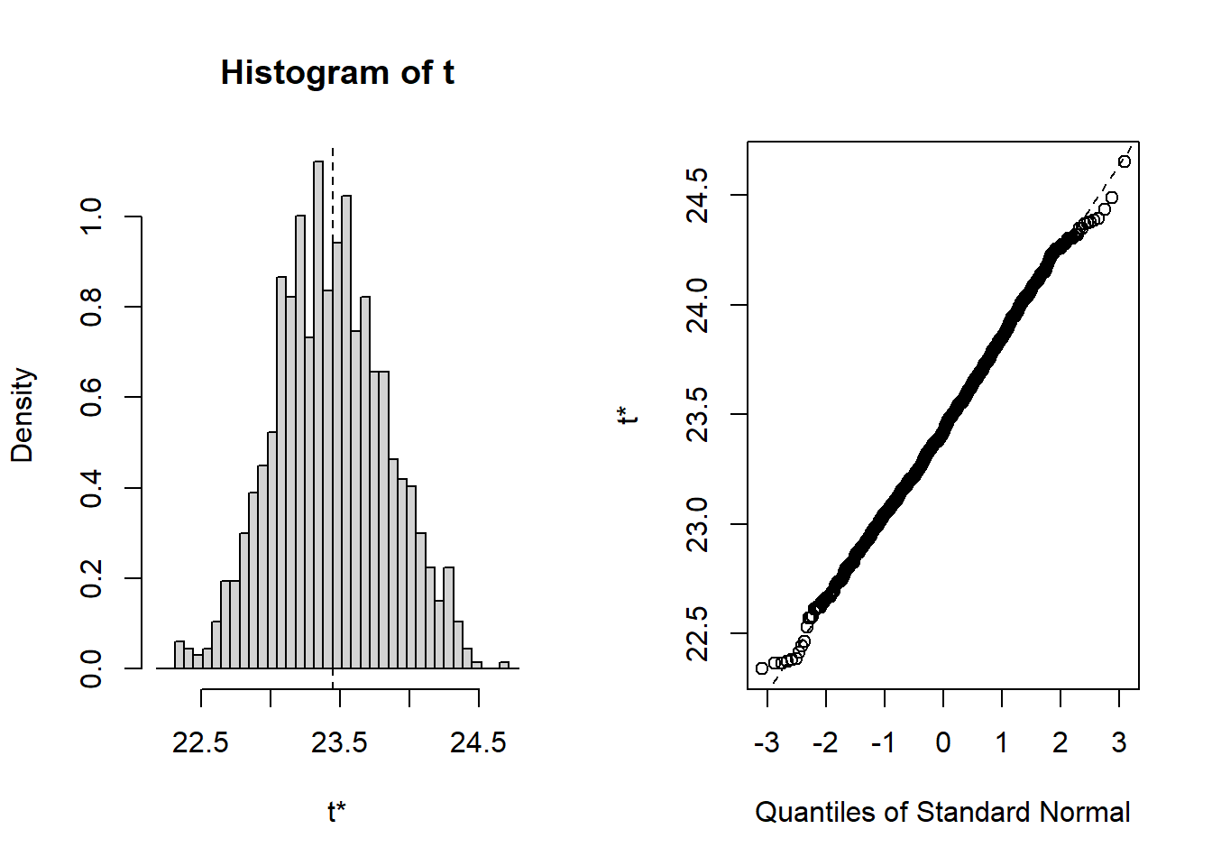

7. Bootstrap for Regression

You can bootstrap regression coefficients as follows:

# Define a statistic to bootstrap coefficients of a linear model
boot_fn <- function(data, indices) {
  sampled_data <- data[indices, ]
  fit <- lm(mpg ~ horsepower, data = sampled_data)
  return(coef(fit))
}

# Perform bootstrapping
set.seed(123)
boot_reg <- boot(data = Auto, statistic = boot_fn, R = 1000)
print(boot_reg)

ORDINARY NONPARAMETRIC BOOTSTRAP


Call:
boot(data = Auto, statistic = boot_fn, R = 1000)


Bootstrap Statistics :
      original        bias    std. error
t1* 39.9358610  0.0156469811 0.845583773
t2* -0.1578447 -0.0001803022 0.007393556

lm(mpg ~ horsepower, data = Auto)  # Original regression coefficients

Call:
lm(formula = mpg ~ horsepower, data = Auto)

Coefficients:
(Intercept)   horsepower  
    39.9359      -0.1578  

8. Interpret the Output

• Bootstrap Estimates: Mean or coefficients calculated across resampled datasets.
• Bias and Standard Error: Provided in the boot result, giving insight into variability.

9. Visualize the Confidence Intervals

For confidence intervals:

boot.ci(boot.out = boot_result, type = c("norm", "basic", "perc", "bca"))

BOOTSTRAP CONFIDENCE INTERVAL CALCULATIONS
Based on 1000 bootstrap replicates

CALL : 
boot.ci(boot.out = boot_result, type = c("norm", "basic", "perc", 
    "bca"))

Intervals : 
Level      Normal              Basic         
95%   (22.67, 24.24 )   (22.64, 24.22 )  

Level     Percentile            BCa          
95%   (22.67, 24.25 )   (22.69, 24.28 )  
Calculations and Intervals on Original Scale

10. Adaptation to Machine Learning

For machine learning tasks like cross-validation or parameter tuning, you can use bootstrapping in similar ways: - Combine bootstrap resampling with algorithms like glm for logistic regression or randomForest for more complex models.