VECM Models

Zahid Asghar

1/8/23

VECM and Cointegration

Macro data are attached herewith.

  • Plot all the series
  • Test for unit root (Use SBIC for lag selection)
  • If all series are non-stationary, use Johansen Cointegration procedure for case-3 option (constant in CE and in LR relation). Appropriate lag length selection is important.
  • Estimate VECM model and forecast it for next 4 quarters
  • Complete the write up and submit it in 1 hour.
  • • Experience the process of practical application of time series analysis.

• Get hands-on experience with the analysis of time series.

• Give correct interpretation of outcomes of the analysis.

Main Objectives

  • Concept of cointegration

  • Studying the dynamics of cointegrated variables

  • Methods for testing cointegration

  • How to estimate a system of cointegrated variables

  • VAR and VECM difference

Money, Prices and GDP

  • Data for money, prices and gdp

  • Purpose is forecasting for next 4 to 8 quarters

Graphs of data

## # A tibble: 204 × 12
##    date...1            quarter Quarter  Year date...5  QRGDP M2_mi…¹ LNRGDP
##    <dttm>                <dbl> <chr>   <dbl> <chr>     <dbl>   <dbl>  <dbl>
##  1 1970-01-01 00:00:00       1 Q1       1970 1970Q1   223168   20800   12.3
##  2 1970-04-01 00:00:00       2 Q2       1970 1970Q2   225140   21500   12.3
##  3 1970-07-01 00:00:00       3 Q3       1970 1970Q3   225980   22213   12.3
##  4 1970-10-01 00:00:00       4 Q4       1970 1970Q4   245436   22965   12.4
##  5 1971-01-01 00:00:00       1 Q1       1971 1971Q1   251348   23632   12.4
##  6 1971-04-01 00:00:00       2 Q2       1971 1971Q2   259999   24643   12.5
##  7 1971-07-01 00:00:00       3 Q3       1971 1971Q3   261355   24718   12.5
##  8 1971-10-01 00:00:00       4 Q4       1971 1971Q4   271232   24300   12.5
##  9 1972-01-01 00:00:00       1 Q1       1972 1972Q1   279965   24324   12.5
## 10 1972-04-01 00:00:00       2 Q2       1972 1972Q2   285432   25134   12.6
## # … with 194 more rows, 4 more variables: LNM2 <dbl>, CPI <dbl>,
## #   inf <dbl>, `inf cpi` <dbl>, and abbreviated variable name ¹​M2_mill_rs

#df11<-df11 %>% filter(quarter>"1970 Q4" & quarter<="2019 Q1")
g1<-ggplot(df11)+aes(x=date,y=qrgdp)+geom_line()
g2<-ggplot(df11)+aes(x=date,y=lnM2)+geom_line()
g3<-ggplot(df11)+aes(x=date,y=CPI)+geom_line()
g1+g2+g3

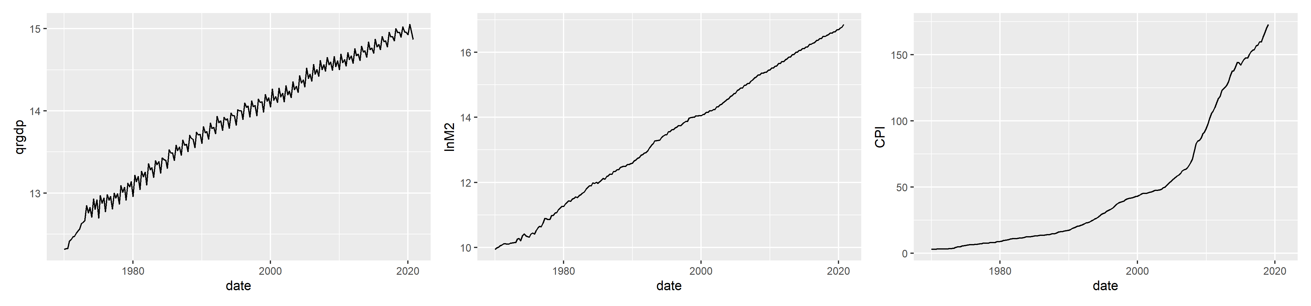
These graphs indicate all three variables are non-stationary.

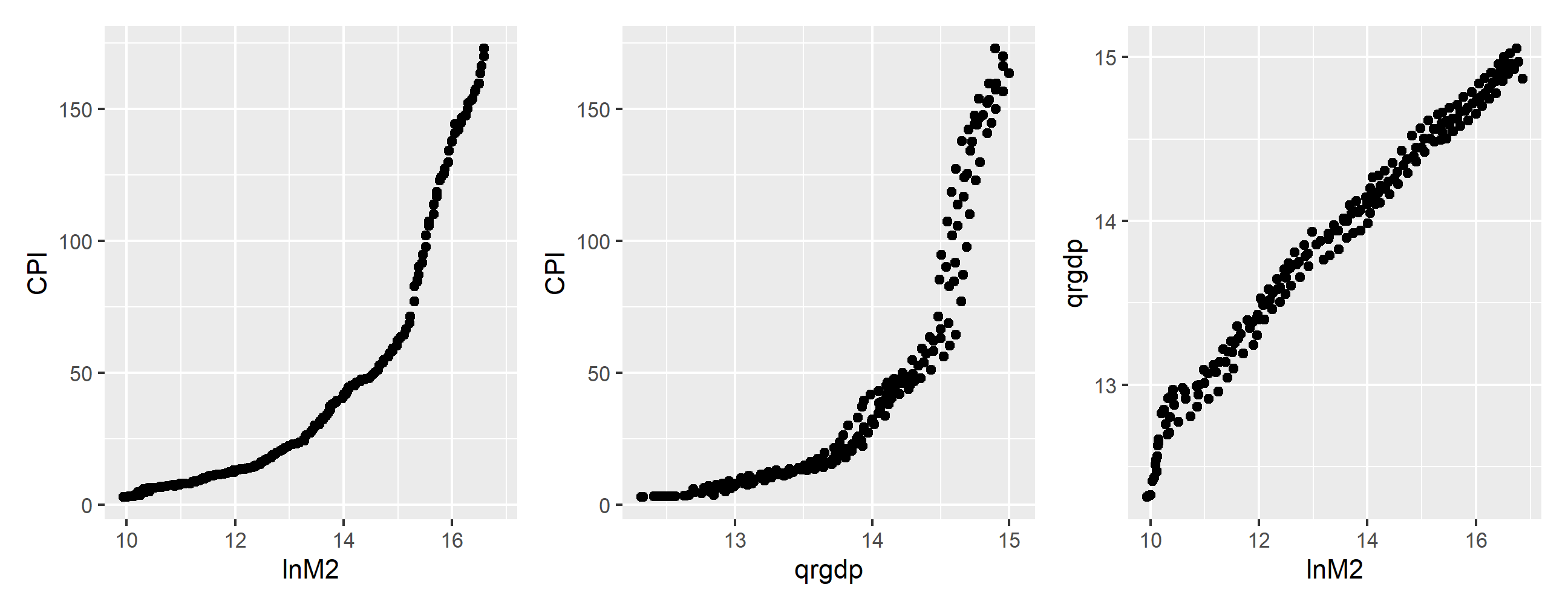
Scatter plot of the variables

Linear Combinations of I(1) series

  • In general a linear combination of I(1) series ) series is also I( 1).
  • However, in some special cases there could be a linear combination which is I(0).
  • So something very special has to happen for a linear combination to become stationary.

Intuition based on theory

  • Usually economic theory helps to find reason why linear combination of I(1) series is stationary I(0).
  • For example Permanent Income Hypothesis, Commodity Market Arbitrage, Purchasing Power Parity
  • Theory guides but one has to test it

What is Cointegration

  • I(1) series are cointegrated if there exists at least one linear combination of these variables which is I(0).

  • In our example _mpy_ if \(b_1m+b_2p+b_3y\) is stationary, there is cointegration.

  • In case variables are nonstationary, usual VAR not a good idea.

  • In case variables are nonstationary but cointegrated, VAR in difference form miss long run dynamics

  • In case variables are nonstationary, not cointegrated, then VAR in difference.

    So lets elaborate more on cointegration and Vector Error Correction models.

Cointegretion and Vector Error Correction Model (VECM)

Money Market equiblibrium \(M^s=M^d=\beta_0+\beta_1p_t+\beta_2y_t+\beta_3r_t+e_t\) \(e_t\) is not persistent and its variance should not rise over time. If \(b_1m+b_2p+b_3y\) is stationary, it means despite each series being non-stationary, their linear combination is stationary and hence these variables are cointegrated.

Long run relationship If \(b_1m+b_2p+b_3y\) is stationary, it means there must be some adjustment made by m,p and y that move together such that deviation from \(b_1m+b_2p+b_3y\)=0 remains bounded.

Money and Price

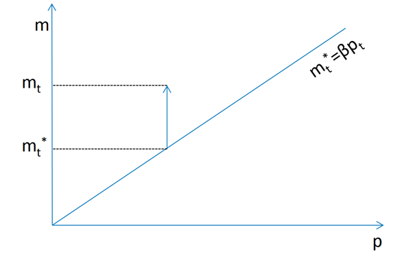
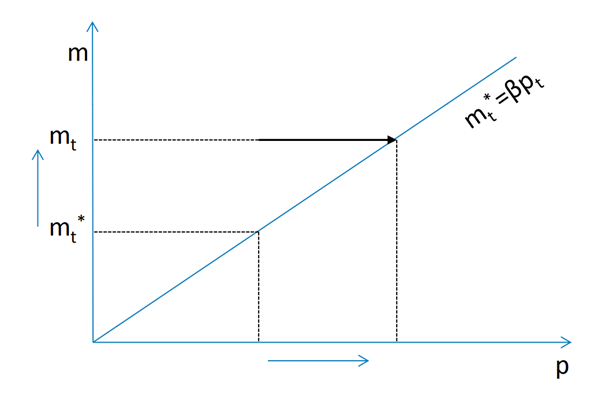
Suppose that in the long run \(m_t=\beta p_t+e_t\) where \(\beta>0\) That is \(m_t\) and \(p_t\) are cointegrated and money nuetrality hypothesis would imply \(\beta=1\). If \(m \uparrow\) s.t \(m_t-\beta p_t>0\), what would be the dynamics?

Deviation and now what

\(m_t\) is doing all the adjument

\(m^*_t\) is unchanged and \(m_t\) \(\downarrow\)

\(\Delta m_t=\alpha_m(m_{t-1}-m^*_{t-1})\) where \(\alpha_m<0\) Short run change in \(m_t\) is a linear function of the deviation from the long run from the long run equilibrium

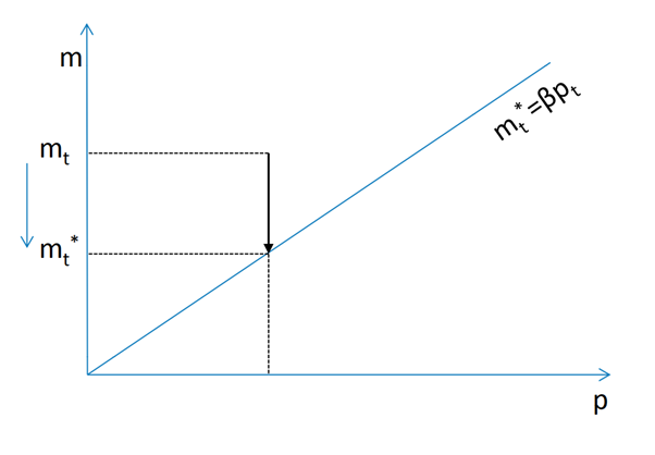
\(m^*_t\) is doing all the adjument

\(m_t\) is unchanged and \(p_t\) and \(m^*_t\) \(\uparrow\) \(\Delta p_t=\alpha_p(m_{t-1}-m^*_{t-1})\) where \(\alpha_p>0\) Short run change in \(p_t\) is a linear function of the deviation from the long run from the long run equilibrium

Both \(m_t\) and \(p_t\) adjust__

\(m_t\) and \(p_t\) are adjusting simultaneously \(\Delta m_t=\alpha_m(m_{t-1}-m^*_{t-1})\) \(\Delta p_t=\alpha_p(m_{t-1}-m^*_{t-1})\) which is basically error/equilibrium correction model. !…

Cointegration and VECM (Continued)

Simple ECM \(m_t\) and \(p_t\) are cointegrated with adjustment in \(e_t\) \(\Delta m_t=\alpha_m(m_{t-1}-\beta p_{t-1})+\nu_t\) \(\Delta p_t=\alpha_p(m_{t-1}-\beta p_{t-1})+\mu_t\) A VAR in difference would be misspecified.

\(m_t=(1+\alpha_m)m_{t-1}-\alpha_m \beta p_{t-1}+\nu_t\)

\(p_t=\alpha_p m_{t-1}-(1-\alpha_p \beta) p_{t-1}+\mu_t\)

These two equations represent VAR but with nonlinear constraints on its coefficients.

Back to money, prices and gdp issue

Economic theory indicate that \(m_t\), \(p_t\) and \(y_t\) are cointegrated. Lets write simple VECM of order zero

No lags of \(\Delta m_t\),\(\Delta p_t\) and \(\Delta y_t\) \(\Delta m_t=\alpha_m(\beta_1 m_{t-1}+\beta_2 p_{t-1}+\beta_3 y_{t-1}+\beta_4)+\nu_t\)

\(\Delta p_t=\alpha_p(\beta_1 m_{t-1}+\beta_2 p_{t-1}+\beta_3 y_{t-1}+\beta_4)+\mu_t\)

\(\Delta y_t=\alpha_y(\beta_1 m_{t-1}+\beta_2 p_{t-1}+\beta_3 y_{t-1}+\beta_4)+\eta_t\)

VECM of order 1

\(\Delta m_t=\alpha_m(\beta_1 m_{t-1}+\beta_2 p_{t-1}+\beta_3 y_{t-1}+\beta_4)+\\ \lambda_{mm} \Delta m_{t-1}+\lambda_{mp} \Delta p_{t-1}+\lambda_{my} \Delta y_{t-1}+\nu_t\)

\(\Delta p_t=\alpha_p(\beta_1 m_{t-1}+\beta_2 p_{t-1}+\beta_3 y_{t-1}+\beta_4)+\\ \lambda_{pm} \Delta m_{t-1}+\lambda_{pp} \Delta p_{t-1}+\lambda_{py} \Delta y_{t-1}\mu_t\)

\(\Delta y_t=\alpha_y(\beta_1 m_{t-1}+\beta_2 p_{t-1}+\beta_3 y_{t-1}+\beta_4)+\\ \lambda_{ym} \Delta m_{t-1}+\lambda_{yp} \Delta p_{t-1}+\lambda_{yy} \Delta y_{t-1}+\eta_t\)

Deterministic component

Case 1 \(\Delta m_t=\alpha_m(\beta_1 m_{t-1}+\beta_2 p_{t-1}+\beta_3 y_{t-1}+)+\\\lambda_{mm} \Delta m_{t-1}+\lambda_{mp} \Delta p_{t-1}+\lambda_{my} \Delta y_{t-1}+\nu_t\)

Case 2

\(\Delta m_t=\alpha_m(\beta_1 m_{t-1}+\beta_2 p_{t-1}+\beta_3 y_{t-1}+\beta_4)+\\\lambda_{mm} \Delta m_{t-1}+\lambda_{mp} \Delta p_{t-1}+\lambda_{my} \Delta y_{t-1}+\nu_t\)

Case 3

\(\Delta m_t=\mu_m+\alpha_m(\beta_1 m_{t-1}+\beta_2 p_{t-1}+\beta_3 y_{t-1}+\beta_4)+\\\lambda_{mm} \Delta m_{t-1}+\lambda_{mp} \Delta p_{t-1}+\lambda_{my} \Delta y_{t-1}+\nu_t\)

Case 3 VECM order 1 with constant

\(\Delta m_t=\mu_m+\alpha_m(\beta_1 m_{t-1}+\beta_2 p_{t-1}+\beta_3 y_{t-1}+\beta_4)+\\\lambda_{mm} \Delta m_{t-1}+\lambda_{mp} \Delta p_{t-1}+\lambda_{my} \Delta y_{t-1}+\nu_t\)

\(\Delta p_t=\mu_p+\alpha_p(\beta_1 m_{t-1}+\beta_2 p_{t-1}+\beta_3 y_{t-1}+\beta_4)+\\\lambda_{pm} \Delta m_{t-1}+\lambda_{pp} \Delta p_{t-1}+\lambda_{py} \Delta y_{t-1}\mu_t\)

\(\Delta y_t=\mu_y+\alpha_y(\beta_1 m_{t-1}+\beta_2 p_{t-1}+\beta_3 y_{t-1}+\beta_4)+\\\lambda_{ym} \Delta m_{t-1}+\lambda_{yp} \Delta p_{t-1}+\lambda_{yy} \Delta y_{t-1}+\eta_t\) VECM in Matric Form

\(\Delta X_t=C+\Pi X_{t-1}+\Lambda \Delta X_{t-1}+e_t\)

\(\Pi X_{t-1}\) represents error correction term

Methods of Cointegration testing

  • Engle Granger two step method
  • Johansen Cointegration procedure Jo.CI rests on estimating rank(\(\Pi\)) which is maximum number of independent vectors it contains.

If rank(\(\Pi\))=0 , no cointegration

If rank(\(\Pi\)) is full, all variables are I(0)

\(0<rank(\Pi)=r<n\) there are \(r\) independent cointegration relationships

Trace Statistics for r:the null hypothesis is that the null hypothesis is that the rank is at most \(r\) vs the rank is strictly greater

Eigen Value Statistics for r:the null hypothesis is that the rank is \(r\) vs. the rank is \(r+1\)

Weak Exogeniety

\(\Delta m_t=\mu_m+\alpha_m(\beta_1 m_{t-1}+\beta_2 p_{t-1}+\beta_3 y_{t-1}+\beta_4)+\\\lambda_{mm} \Delta m_{t-1}+\lambda_{mp} \Delta p_{t-1}+\lambda_{my} \Delta y_{t-1}+\nu_t\)

\(\Delta p_t=\mu_p+\alpha_p(\beta_1 m_{t-1}+\beta_2 p_{t-1}+\beta_3 y_{t-1}+\beta_4)+\\\lambda_{pm} \Delta m_{t-1}+\lambda_{pp} \Delta p_{t-1}+\lambda_{py} \Delta y_{t-1}\mu_t\)

\(\Delta y_t=\mu_y+\alpha_y(\beta_1 m_{t-1}+\beta_2 p_{t-1}+\beta_3 y_{t-1}+\beta_4)+\\\lambda_{ym} \Delta m_{t-1}+\lambda_{yp} \Delta p_{t-1}+\lambda_{yy} \Delta y_{t-1}+\eta_t\)

Testing \(\alpha_y=0\) implies \(y_t\) is weakly exogenous.