Demographic Analysis Using R

Population & Health Data with Tidyverse

Zahid Asghar, School of Economics, QAU

2026-08-30

Welcome to Demographic Data Analysis!

What You’ll Learn Today

• Import and explore health/demographic data
• Clean and transform population datasets
• Calculate demographic indicators
• Analyze health outcomes by age, sex, and socioeconomic factors
• Create reproducible demographic reports
• Visualize population health patterns

Note

We’ll use real NHANES data - the same type used by demographers and public health researchers worldwide

About NHANES Data

National Health and Nutrition Examination Survey (NHANES)

• Conducted by CDC (USA)
• Representative sample of US population
• Combines interviews + physical examinations
• Gold standard for health surveillance

Today’s variables:

• Demographics: Age, Sex, Race, Education
• Anthropometric: Height, Weight, BMI
• Health: Blood Pressure, Diabetes, Physical Activity
• Socioeconomic: Poverty, Insurance

Why R for Demographic Analysis?

R Advantages:

✅ Purpose-built for statistics
✅ Excellent for survey data
✅ Powerful visualization
✅ Reproducible reports
✅ Free and open source
✅ Growing demographic/health community

Common Tasks:

• Population pyramids
• Age-standardization
• Fertility/mortality analysis
• Health inequality assessment
• Survey data analysis
• Cohort studies

Our Analytical Journey Today

flowchart LR
    A[Import Data] --> B[Explore & Clean]
    B --> C[Transform Variables]
    C --> D[Calculate Indicators]
    D --> E[Analyze Patterns]
    E --> F[Visualize Results]
    F --> G[Report Findings]
    
    style A fill:#e1f5dd
    style G fill:#ffd6d6

flowchart LR
    A[Import Data] --> B[Explore & Clean]
    B --> C[Transform Variables]
    C --> D[Calculate Indicators]
    D --> E[Analyze Patterns]
    E --> F[Visualize Results]
    F --> G[Report Findings]
    
    style A fill:#e1f5dd
    style G fill:#ffd6d6

Part 1: Getting Started

Loading Packages

library(tidyverse)    # Data wrangling & visualization
library(rio)          # Import/export any format
library(modelsummary) # Summary tables
library(NHANES)       # Our practice dataset

Tip

Install packages first if needed:

install.packages(c("tidyverse", "rio", "modelsummary", "NHANES"))

Loading NHANES Data

# Load NHANES dataset
data("NHANES")

# Create a clean working dataset
nhanes_data <- NHANES %>%
  as_tibble() %>%
  # Select relevant variables for demographic analysis
  select(
    # Demographics
    ID, Gender, Age, AgeDecade, Race1, Education, 
    MaritalStatus, HomeOwn,
    # Health measures
    Height, Weight, BMI, BPSysAve, BPDiaAve,
    Diabetes, PhysActive, SmokeNow,
    # Socioeconomic
    HHIncome, Poverty
  ) %>%
  # Remove duplicates (NHANES has some repeated IDs)
  distinct(ID, .keep_all = TRUE)

First Look at Our Data

glimpse(nhanes_data)

Rows: 6,779
Columns: 18
$ ID            <int> 51624, 51625, 51630, 51638, 51646, 51647, 51654, 51656, …
$ Gender        <fct> male, male, female, male, male, female, male, male, male…
$ Age           <int> 34, 4, 49, 9, 8, 45, 66, 58, 54, 10, 58, 50, 9, 33, 60, …
$ AgeDecade     <fct>  30-39,  0-9,  40-49,  0-9,  0-9,  40-49,  60-69,  50-59…
$ Race1         <fct> White, Other, White, White, White, White, White, White, …
$ Education     <fct> High School, NA, Some College, NA, NA, College Grad, Som…
$ MaritalStatus <fct> Married, NA, LivePartner, NA, NA, Married, Married, Divo…
$ HomeOwn       <fct> Own, Own, Rent, Rent, Own, Own, Own, Rent, Rent, Own, Re…
$ Height        <dbl> 164.7, 105.4, 168.4, 133.1, 130.6, 166.7, 169.5, 181.9, …
$ Weight        <dbl> 87.4, 17.0, 86.7, 29.8, 35.2, 75.7, 68.0, 78.4, 74.7, 38…
$ BMI           <dbl> 32.22, 15.30, 30.57, 16.82, 20.64, 27.24, 23.67, 23.69, …
$ BPSysAve      <int> 113, NA, 112, 86, 107, 118, 111, 104, 134, 104, 127, 142…
$ BPDiaAve      <int> 85, NA, 75, 47, 37, 64, 63, 74, 85, 68, 83, 68, 63, 74, …
$ Diabetes      <fct> No, No, No, No, No, No, No, No, No, No, No, No, No, No, …
$ PhysActive    <fct> No, NA, No, NA, NA, Yes, Yes, Yes, Yes, NA, Yes, Yes, NA…
$ SmokeNow      <fct> No, NA, Yes, NA, NA, NA, No, NA, NA, NA, Yes, NA, NA, No…
$ HHIncome      <fct> 25000-34999, 20000-24999, 35000-44999, 75000-99999, 5500…
$ Poverty       <dbl> 1.36, 1.07, 1.91, 1.84, 2.33, 5.00, 2.20, 5.00, 2.20, NA…

Data Overview

# How many observations?
nrow(nhanes_data)

[1] 6779

# Summary statistics
datasummary_skim(nhanes_data, histogram = FALSE)

	Unique	Missing Pct.	Mean	SD	Min	Median	Max
ID	6779	0	61657.2	5869.4	51624.0	61615.0	71915.0
Age	81	0	35.5	23.1	0.0	34.0	80.0
Height	981	4	160.4	21.1	83.6	165.1	200.4
Weight	1291	1	69.1	29.9	2.8	71.1	230.7
BMI	2074	4	26.5	7.5	12.9	25.8	81.2
BPSysAve	127	17	118.0	17.6	76.0	116.0	226.0
BPDiaAve	103	17	66.7	14.9	0.0	68.0	116.0
Poverty	451	8	2.6	1.7	0.0	2.3	5.0
		N	%
Gender	female	3420	50.4
	male	3359	49.6
AgeDecade	0-9	1109	16.4
	10-19	1016	15.0
	20-29	880	13.0
	30-39	895	13.2
	40-49	845	12.5
	50-59	768	11.3
	60-69	601	8.9
	70+	416	6.1
Race1	Black	1024	15.1
	Hispanic	495	7.3
	Mexican	859	12.7
	White	3783	55.8
	Other	618	9.1
Education	8th Grade	359	5.3
	9 - 11th Grade	624	9.2
	High School	993	14.6
	Some College	1423	21.0
	College Grad	1246	18.4
MaritalStatus	Divorced	443	6.5
	LivePartner	374	5.5
	Married	2463	36.3
	NeverMarried	899	13.3
	Separated	135	2.0
	Widowed	336	5.0
HomeOwn	Own	4149	61.2
	Rent	2419	35.7
	Other	167	2.5
Diabetes	No	6101	90.0
	Yes	552	8.1
PhysActive	No	2473	36.5
	Yes	2972	43.8
SmokeNow	No	1092	16.1
	Yes	964	14.2
HHIncome	0-4999	159	2.3
	5000-9999	199	2.9
	10000-14999	425	6.3
	15000-19999	409	6.0
	20000-24999	476	7.0
	25000-34999	689	10.2
	35000-44999	608	9.0
	45000-54999	511	7.5
	55000-64999	390	5.8
	65000-74999	334	4.9
	75000-99999	691	10.2
	more 99999	1303	19.2

Understanding Our Variables

Demographics:

• Age: Continuous age in years
• Gender: Male/Female
• Race1: Race/ethnicity categories
• Education: Educational attainment

Health Indicators:

• BMI: Body Mass Index (kg/m²)
• BPSysAve: Systolic blood pressure
• Diabetes: Yes/No
• PhysActive: Physically active (Yes/No)

Socioeconomic:

• HHIncome: Household income categories
• Poverty: Income-to-poverty ratio

Part 2: Data Exploration

Basic Demographic Profile

nhanes_data %>%
  summarise(
    n = n(),
    avg_age = mean(Age, na.rm = TRUE),
    pct_female = mean(Gender == "female", na.rm = TRUE) * 100,
    pct_diabetes = mean(Diabetes == "Yes", na.rm = TRUE) * 100
  )

Age Distribution

nhanes_data %>%
  count(AgeDecade) %>%
  mutate(
    percentage = n / sum(n) * 100,
    percentage = round(percentage, 1)
  ) %>%
  arrange(AgeDecade)

Gender Distribution

nhanes_data %>%
  count(Gender) %>%
  mutate(
    percentage = n / sum(n) * 100,
    percentage = round(percentage, 1)
  )

Checking for Missing Data

nhanes_data %>%
  summarise(
    across(
      c(Age, Gender, BMI, BPSysAve, Diabetes),
      ~ sum(is.na(.)) / n() * 100
    )
  ) %>%
  pivot_longer(everything(), 
               names_to = "variable",
               values_to = "pct_missing") %>%
  mutate(pct_missing = round(pct_missing, 1))

Part 3: Data Cleaning & Transformation

Creating Age Groups

nhanes_clean <- nhanes_data %>%
  mutate(
    # Create standard demographic age groups
    age_group = case_when(
      Age < 18 ~ "0-17",
      Age >= 18 & Age < 35 ~ "18-34",
      Age >= 35 & Age < 50 ~ "35-49",
      Age >= 50 & Age < 65 ~ "50-64",
      Age >= 65 ~ "65+",
      TRUE ~ NA_character_
    ),
    # Convert to factor with correct order
    age_group = factor(age_group, 
                      levels = c("0-17", "18-34", "35-49", 
                                "50-64", "65+"))
  )

Creating Health Indicators

nhanes_clean <- nhanes_clean %>%
  mutate(
    # BMI categories (WHO classification)
    bmi_category = case_when(
      BMI < 18.5 ~ "Underweight",
      BMI >= 18.5 & BMI < 25 ~ "Normal",
      BMI >= 25 & BMI < 30 ~ "Overweight",
      BMI >= 30 ~ "Obese",
      TRUE ~ NA_character_
    ),
    bmi_category = factor(bmi_category,
                         levels = c("Underweight", "Normal", 
                                   "Overweight", "Obese")),
    
    # Hypertension (BP >= 140/90)
    hypertension = case_when(
      BPSysAve >= 140 | BPDiaAve >= 90 ~ "Yes",
      !is.na(BPSysAve) & !is.na(BPDiaAve) ~ "No",
      TRUE ~ NA_character_
    )
  )

Creating Socioeconomic Variables

nhanes_clean <- nhanes_clean %>%
  mutate(
    # Education level (simplified)
    education_level = case_when(
      Education %in% c("8th Grade", "9 - 11th Grade") ~ "Less than HS",
      Education == "High School" ~ "High School",
      Education == "Some College" ~ "Some College",
      Education == "College Grad" ~ "College+",
      TRUE ~ NA_character_
    ),
    education_level = factor(education_level,
                            levels = c("Less than HS", "High School",
                                      "Some College", "College+")),
    
    # Poverty status
    poverty_status = case_when(
      Poverty < 1 ~ "Below poverty",
      Poverty >= 1 & Poverty < 2 ~ "Near poverty",
      Poverty >= 2 ~ "Above poverty",
      TRUE ~ NA_character_
    )
  )

Verifying Our Transformations

nhanes_clean %>%
  select(Age, age_group, BMI, bmi_category, 
         Education, education_level) %>%
  head(5)

Part 4: Demographic Analysis

Population Structure by Age and Sex

nhanes_clean %>%
  count(age_group, Gender) %>%
  group_by(age_group) %>%
  mutate(
    total = sum(n),
    percentage = n / total * 100
  ) %>%
  select(age_group, Gender, n, percentage)

Age-Specific Health Indicators

nhanes_clean %>%
  filter(!is.na(age_group), !is.na(Diabetes)) %>%
  group_by(age_group) %>%
  summarise(
    n = n(),
    diabetes_prev = mean(Diabetes == "Yes", na.rm = TRUE) * 100,
    avg_bmi = mean(BMI, na.rm = TRUE),
    avg_sbp = mean(BPSysAve, na.rm = TRUE)
  ) %>%
  mutate(across(where(is.numeric), ~round(., 1)))

Health by Gender

nhanes_clean %>%
  group_by(Gender) %>%
  summarise(
    n = n(),
    avg_age = mean(Age, na.rm = TRUE),
    avg_bmi = mean(BMI, na.rm = TRUE),
    diabetes_pct = mean(Diabetes == "Yes", na.rm = TRUE) * 100,
    phys_active_pct = mean(PhysActive == "Yes", na.rm = TRUE) * 100,
    smoker_pct = mean(SmokeNow == "Yes", na.rm = TRUE) * 100
  ) %>%
  mutate(across(where(is.numeric), ~round(., 1)))

Socioeconomic Gradients in Health

nhanes_clean %>%
  filter(!is.na(education_level), !is.na(Diabetes)) %>%
  group_by(education_level) %>%
  summarise(
    n = n(),
    diabetes_prev = mean(Diabetes == "Yes", na.rm = TRUE) * 100,
    obesity_prev = mean(bmi_category == "Obese", na.rm = TRUE) * 100,
    phys_active = mean(PhysActive == "Yes", na.rm = TRUE) * 100
  ) %>%
  mutate(across(where(is.numeric), ~round(., 1)))

BMI Distribution by Age Group

nhanes_clean %>%
  filter(!is.na(age_group), !is.na(bmi_category)) %>%
  count(age_group, bmi_category) %>%
  group_by(age_group) %>%
  mutate(
    percentage = n / sum(n) * 100,
    percentage = round(percentage, 1)
  ) %>%
  arrange(age_group, bmi_category)

Hypertension Prevalence by Age

nhanes_clean %>%
  filter(!is.na(age_group), !is.na(hypertension)) %>%
  group_by(age_group) %>%
  summarise(
    n = n(),
    hypertension_prev = mean(hypertension == "Yes") * 100,
    avg_sbp = mean(BPSysAve, na.rm = TRUE),
    avg_dbp = mean(BPDiaAve, na.rm = TRUE)
  ) %>%
  mutate(across(where(is.numeric), ~round(., 1)))

Part 5: Advanced Analysis

Multiple Group Comparisons

Diabetes prevalence by age, gender, and education:

nhanes_clean %>%
  filter(
    !is.na(age_group),
    !is.na(Gender),
    !is.na(education_level),
    !is.na(Diabetes)
  ) %>%
  group_by(age_group, Gender, education_level) %>%
  summarise(
    n = n(),
    diabetes_prev = mean(Diabetes == "Yes") * 100,
    .groups = "drop"
  ) %>%
  filter(n >= 20) %>%  # Only groups with 20+ observations
  arrange(age_group, Gender, education_level) %>%
  head(10)

Creating Summary Tables

health_summary <- nhanes_clean %>%
  filter(!is.na(Gender), !is.na(age_group)) %>%
  group_by(Gender, age_group) %>%
  summarise(
    N = n(),
    `Mean Age` = round(mean(Age, na.rm = TRUE), 1),
    `Mean BMI` = round(mean(BMI, na.rm = TRUE), 1),
    `Diabetes (%)` = round(mean(Diabetes == "Yes", na.rm = TRUE) * 100, 1),
    `Hypertension (%)` = round(mean(hypertension == "Yes", na.rm = TRUE) * 100, 1),
    .groups = "drop"
  )

Health Summary Table

head(health_summary, 10)

Calculating Prevalence Ratios

Example: Diabetes prevalence by education (reference: College+)

# Calculate prevalence by education
diabetes_by_ed <- nhanes_clean %>%
  filter(!is.na(education_level), !is.na(Diabetes)) %>%
  group_by(education_level) %>%
  summarise(
    prevalence = mean(Diabetes == "Yes") * 100
  )

# Calculate prevalence ratios
diabetes_by_ed %>%
  mutate(
    reference_prev = prevalence[education_level == "College+"],
    prevalence_ratio = prevalence / reference_prev
  ) %>%
  mutate(across(where(is.numeric), ~round(., 2)))

Age Standardization Example

Simple direct standardization:

# Reference population (all ages)
reference_age_dist <- nhanes_clean %>%
  count(age_group) %>%
  mutate(weight = n / sum(n))

# Age-specific rates by gender
age_specific_rates <- nhanes_clean %>%
  filter(!is.na(Diabetes), !is.na(age_group)) %>%
  group_by(Gender, age_group) %>%
  summarise(
    rate = mean(Diabetes == "Yes") * 100,
    .groups = "drop"
  )

# Standardized rates
age_specific_rates %>%
  left_join(reference_age_dist, by = "age_group") %>%
  group_by(Gender) %>%
  summarise(
    crude_rate = mean(rate),
    standardized_rate = sum(rate * weight),
    .groups = "drop"
  ) %>%
  mutate(across(where(is.numeric), ~round(., 2)))

Part 6: Data Visualization

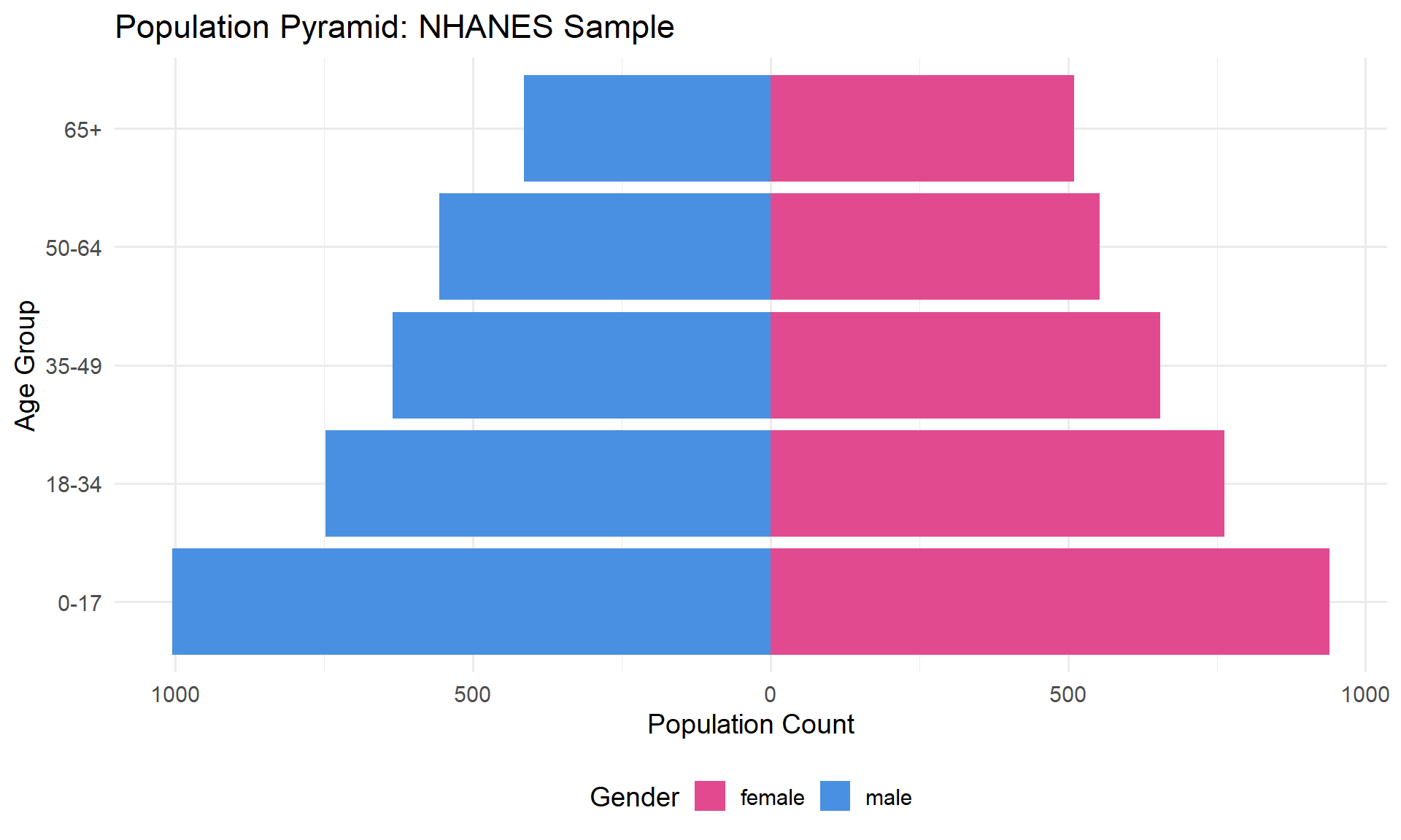
Population Pyramid

nhanes_clean %>%
  filter(!is.na(age_group), !is.na(Gender)) %>%
  count(age_group, Gender) %>%
  mutate(
    n = ifelse(Gender == "male", -n, n)
  ) %>%
  ggplot(aes(x = age_group, y = n, fill = Gender)) +
  geom_col() +
  coord_flip() +
  scale_y_continuous(
    labels = abs,
    name = "Population Count"
  ) +
  scale_fill_manual(values = c("male" = "#4A90E2", "female" = "#E24A90")) +
  labs(
    title = "Population Pyramid: NHANES Sample",
    x = "Age Group",
    fill = "Gender"
  ) +
  theme_minimal(base_size = 14) +
  theme(legend.position = "bottom")

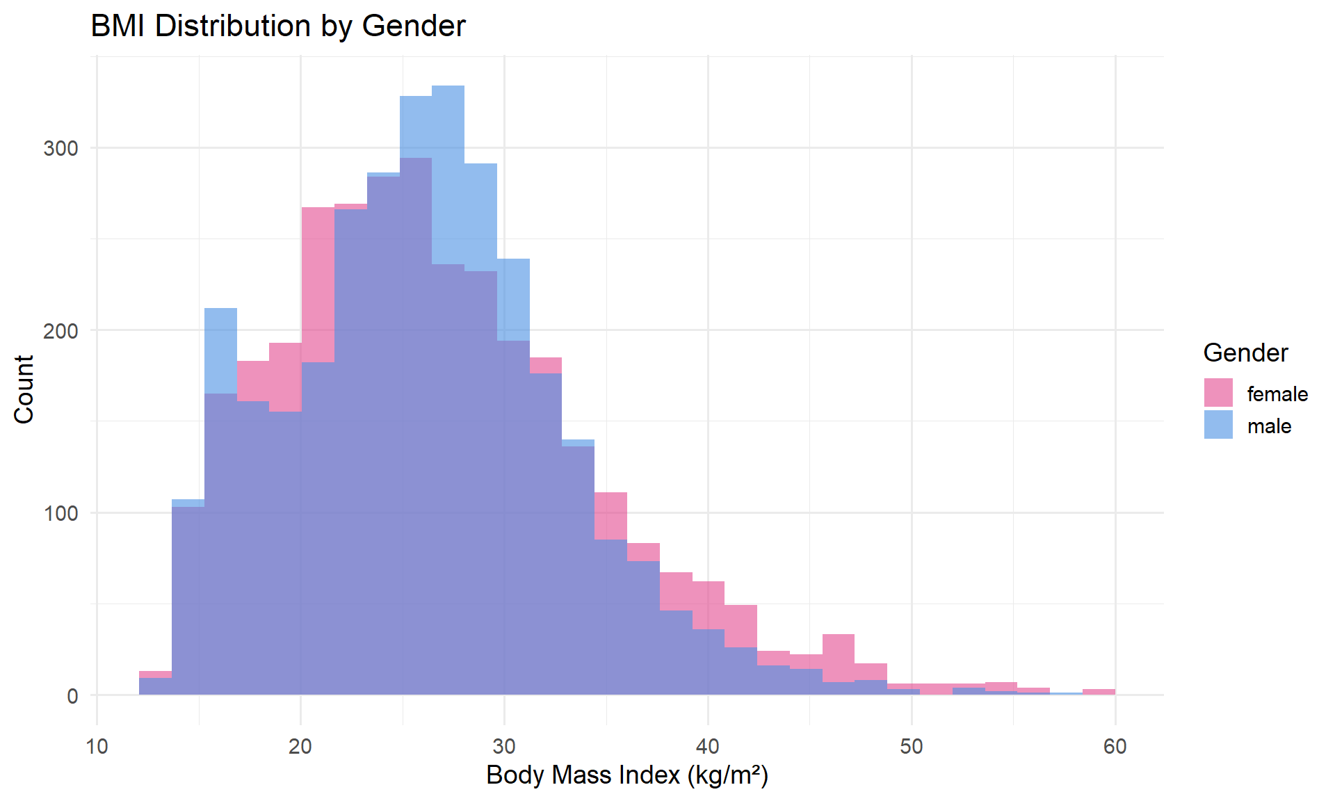
BMI Distribution

nhanes_clean %>%
  filter(!is.na(BMI), BMI < 60) %>%
  ggplot(aes(x = BMI, fill = Gender)) +
  geom_histogram(bins = 30, alpha = 0.6, position = "identity") +
  scale_fill_manual(values = c("male" = "#4A90E2", "female" = "#E24A90")) +
  labs(
    title = "BMI Distribution by Gender",
    x = "Body Mass Index (kg/m²)",
    y = "Count"
  ) +
  theme_minimal(base_size = 14)

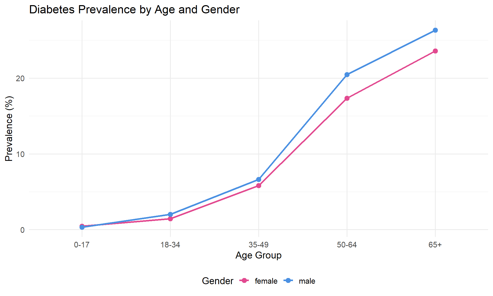
Diabetes Prevalence by Age

nhanes_clean %>%
  filter(!is.na(age_group), !is.na(Diabetes)) %>%
  group_by(age_group, Gender) %>%
  summarise(
    prevalence = mean(Diabetes == "Yes") * 100,
    .groups = "drop"
  ) %>%
  ggplot(aes(x = age_group, y = prevalence, 
             color = Gender, group = Gender)) +
  geom_line(size = 1.2) +
  geom_point(size = 3) +
  scale_color_manual(values = c("male" = "#4A90E2", "female" = "#E24A90")) +
  labs(
    title = "Diabetes Prevalence by Age and Gender",
    x = "Age Group",
    y = "Prevalence (%)"
  ) +
  theme_minimal(base_size = 14) +
  theme(legend.position = "bottom")

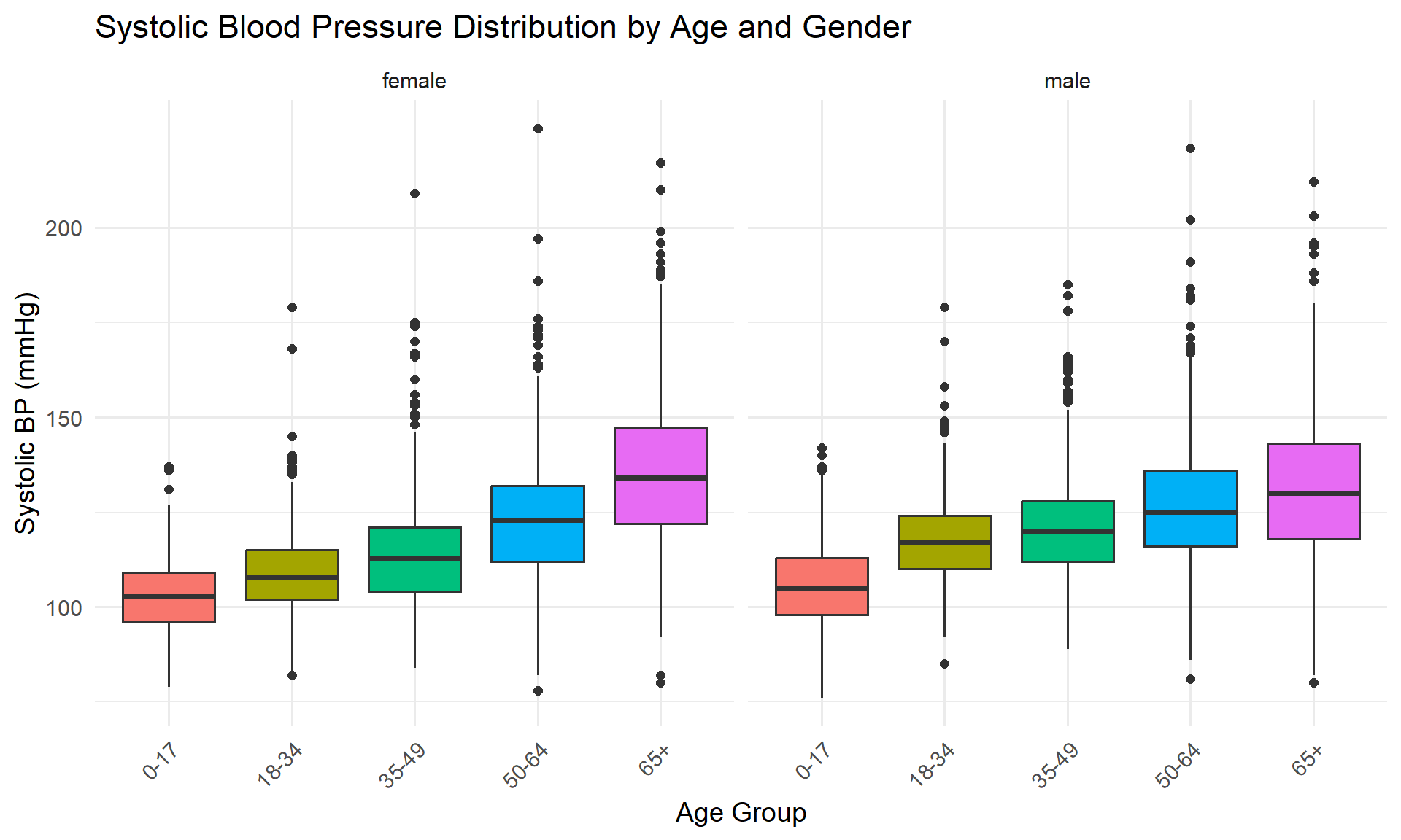
Blood Pressure by Age

nhanes_clean %>%
  filter(!is.na(age_group), !is.na(BPSysAve)) %>%
  ggplot(aes(x = age_group, y = BPSysAve, fill = age_group)) +
  geom_boxplot() +
  facet_wrap(~Gender) +
  labs(
    title = "Systolic Blood Pressure Distribution by Age and Gender",
    x = "Age Group",
    y = "Systolic BP (mmHg)"
  ) +
  theme_minimal(base_size = 14) +
  theme(
    legend.position = "none",
    axis.text.x = element_text(angle = 45, hjust = 1)
  )

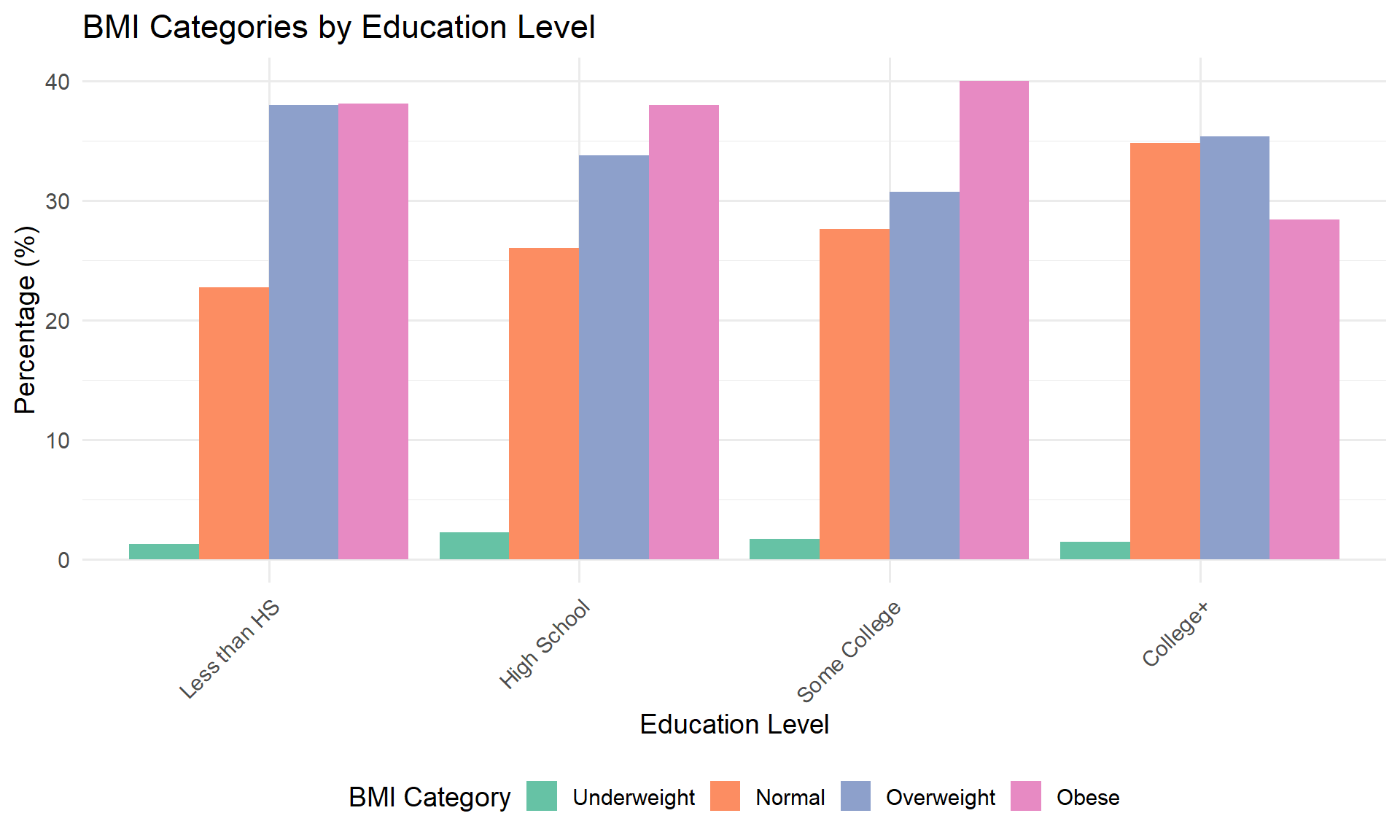
Education and Health

nhanes_clean %>%
  filter(!is.na(education_level), !is.na(bmi_category)) %>%
  count(education_level, bmi_category) %>%
  group_by(education_level) %>%
  mutate(percentage = n / sum(n) * 100) %>%
  ggplot(aes(x = education_level, y = percentage, fill = bmi_category)) +
  geom_col(position = "dodge") +
  scale_fill_brewer(palette = "Set2") +
  labs(
    title = "BMI Categories by Education Level",
    x = "Education Level",
    y = "Percentage (%)",
    fill = "BMI Category"
  ) +
  theme_minimal(base_size = 14) +
  theme(
    axis.text.x = element_text(angle = 45, hjust = 1),
    legend.position = "bottom"
  )

Part 7: Practical Exercises

Exercise 1: Basic Analysis

Task: Calculate obesity prevalence by race/ethnicity

# Your code here
nhanes_clean %>%
  filter(!is.na(___), !is.na(___)) %>%
  group_by(___) %>%
  summarise(
    n = ___,
    obesity_prev = mean(___ == "___") * 100
  )

Exercise 1: Solution

nhanes_clean %>%
  filter(!is.na(Race1), !is.na(bmi_category)) %>%
  group_by(Race1) %>%
  summarise(
    n = n(),
    obesity_prev = mean(bmi_category == "Obese") * 100
  ) %>%
  arrange(desc(obesity_prev)) %>%
  mutate(obesity_prev = round(obesity_prev, 1))

Exercise 2: Multiple Variables

Task: Analyze physical activity by age group and poverty status

# Your code here
nhanes_clean %>%
  filter(!is.na(___), !is.na(___), !is.na(___)) %>%
  group_by(___, ___) %>%
  summarise(
    active_pct = ___,
    .groups = "drop"
  )

Exercise 2: Solution

nhanes_clean %>%
  filter(
    !is.na(age_group),
    !is.na(poverty_status),
    !is.na(PhysActive)
  ) %>%
  group_by(age_group, poverty_status) %>%
  summarise(
    n = n(),
    active_pct = mean(PhysActive == "Yes") * 100,
    .groups = "drop"
  ) %>%
  filter(n >= 20) %>%
  mutate(active_pct = round(active_pct, 1)) %>%
  arrange(age_group, poverty_status)

Exercise 3: Create Visualization

Task: Create a bar chart of hypertension prevalence by age group

# Your code here
nhanes_clean %>%
  filter(!is.na(___), !is.na(___)) %>%
  group_by(___) %>%
  summarise(prev = ___) %>%
  ggplot(aes(x = ___, y = ___)) +
  geom_col(fill = "steelblue") +
  labs(title = "___")

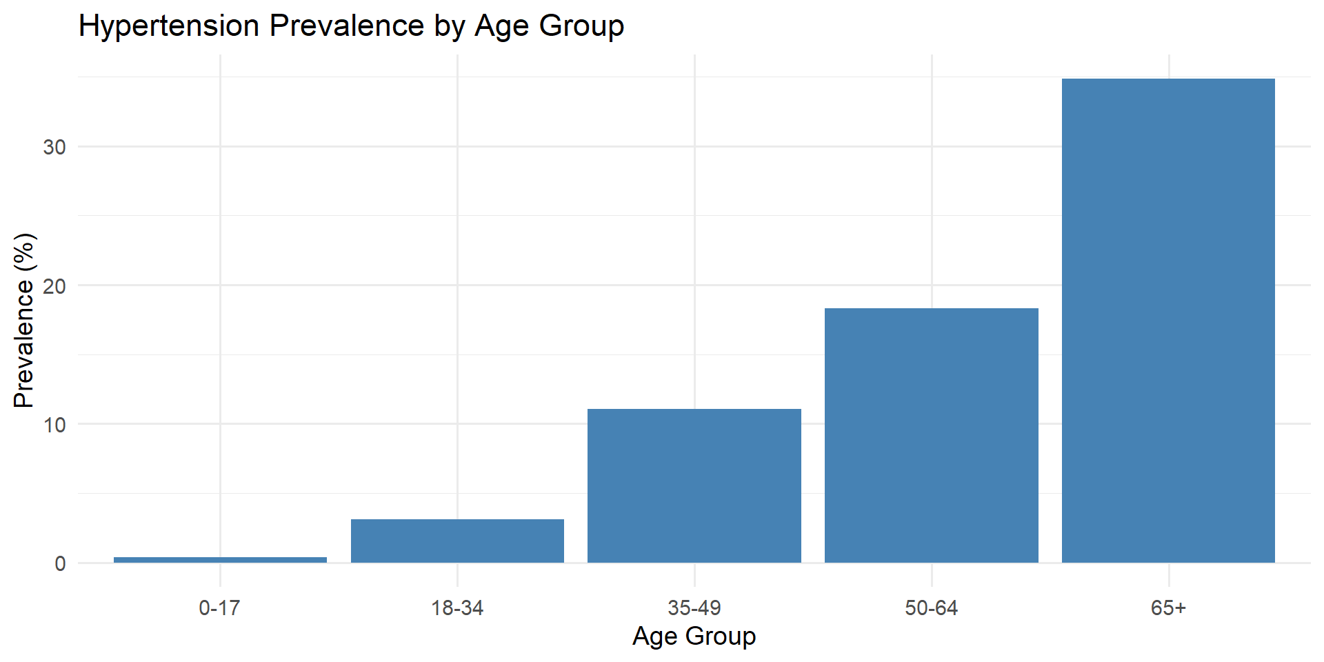
Exercise 3: Solution

nhanes_clean %>%
  filter(!is.na(age_group), !is.na(hypertension)) %>%
  group_by(age_group) %>%
  summarise(prev = mean(hypertension == "Yes") * 100) %>%
  ggplot(aes(x = age_group, y = prev)) +
  geom_col(fill = "steelblue") +
  labs(
    title = "Hypertension Prevalence by Age Group",
    x = "Age Group",
    y = "Prevalence (%)"
  ) +
  theme_minimal(base_size = 14)

Exercise 4: Complex Analysis

Task: Compare mean BMI across education levels, separately for each gender and age group (adults only)

Hints:

1. Filter for adults (Age >= 18)
2. Remove missing values
3. Group by three variables
4. Calculate mean BMI
5. Filter for groups with n >= 10

Exercise 4: Solution

nhanes_clean %>%
  filter(
    Age >= 18,
    !is.na(education_level),
    !is.na(Gender),
    !is.na(age_group),
    !is.na(BMI)
  ) %>%
  group_by(Gender, age_group, education_level) %>%
  summarise(
    n = n(),
    mean_bmi = mean(BMI),
    .groups = "drop"
  ) %>%
  filter(n >= 10) %>%
  mutate(mean_bmi = round(mean_bmi, 1)) %>%
  arrange(Gender, age_group, education_level) %>%
  head(12)

Part 8: Exporting Results

Saving Cleaned Data

# Save as CSV
export(nhanes_clean, "nhanes_cleaned.csv")

# Save as RDS (preserves R object types)
export(nhanes_clean, "nhanes_cleaned.rds")

# Save as Stata file
export(nhanes_clean, "nhanes_cleaned.dta")

# Save as Excel
export(nhanes_clean, "nhanes_cleaned.xlsx")

Exporting Summary Tables

# Create summary
summary_table <- nhanes_clean %>%
  group_by(Gender, age_group) %>%
  summarise(
    N = n(),
    `Mean BMI` = mean(BMI, na.rm = TRUE),
    `Diabetes (%)` = mean(Diabetes == "Yes", na.rm = TRUE) * 100,
    .groups = "drop"
  )

# Export
export(summary_table, "health_summary.csv")
export(summary_table, "health_summary.xlsx")

Saving Plots

# Create plot
p <- nhanes_clean %>%
  filter(!is.na(age_group), !is.na(Diabetes)) %>%
  group_by(age_group) %>%
  summarise(prev = mean(Diabetes == "Yes") * 100) %>%
  ggplot(aes(x = age_group, y = prev)) +
  geom_col(fill = "steelblue") +
  labs(title = "Diabetes Prevalence by Age")

# Save
ggsave("diabetes_by_age.png", p, width = 10, height = 6, dpi = 300)
ggsave("diabetes_by_age.pdf", p, width = 10, height = 6)

Best Practices for Demographic Analysis

Data Quality Checks

1. Check for missing data
   • Use summary() or datasummary_skim()
   • Decide on handling strategy (remove, impute, analyze separately)
2. Verify coding
   • Check factor levels: levels(data$variable)
   • Confirm numeric ranges: range(data$variable, na.rm = TRUE)
3. Look for outliers
   • Use boxplots and summary statistics
   • Investigate extreme values
4. Check sample sizes
   • Ensure adequate n in each group
   • Consider combining categories if needed

Analytical Best Practices

1. Age-standardize when comparing populations
   • Different age structures can confound comparisons
2. Report confidence intervals
   • Not just point estimates
3. Consider survey weights
   • If using complex survey data
4. Document your decisions
   • Keep code comments
   • Note any exclusions or transformations
5. Create reproducible workflows
   • Use R scripts or Quarto documents
   • Include session info: sessionInfo()

Visualization Best Practices

1. Choose appropriate chart types
   • Population pyramids for age-sex structure
   • Line charts for trends
   • Bar charts for comparisons
2. Use clear labels
   • Title, axis labels, legend
   • Include sample size where relevant
3. Color considerations
   • Use colorblind-friendly palettes
   • Avoid red-green combinations
4. Keep it simple
   • One clear message per chart
   • Avoid chartjunk

Common Pitfalls to Avoid

Watch Out For:

❌ Simpson’s Paradox - Always consider confounders
❌ Small sample sizes - n < 30 can be unreliable
❌ Multiple testing - Adjust p-values if doing many tests
❌ Correlation ≠ Causation - Be careful with language
❌ Selection bias - Who’s included/excluded?
❌ Ignoring missing data - Can introduce bias
❌ Over-interpretation - Don’t overstate findings

Real-World Applications

Demographic Research Questions

Population Health:

• What is the obesity prevalence in different age groups?
• How does diabetes vary by socioeconomic status?
• Are there gender differences in cardiovascular risk?

Health Inequalities:

• Do education gradients in health exist?
• How do health outcomes vary by race/ethnicity?
• What is the urban-rural health gap?

Policy Relevant:

• Which populations need targeted interventions?
• How effective are prevention programs?
• What are priority health issues for different age groups?

Example: Health Inequality Report

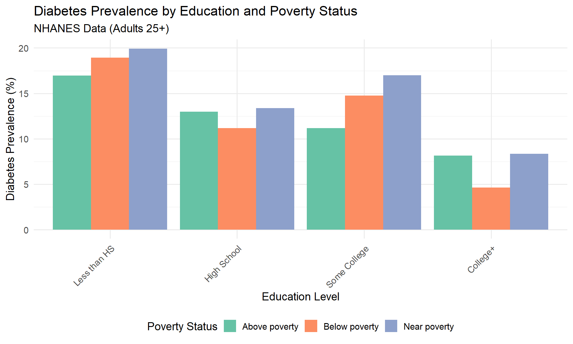
Research Question: How does diabetes prevalence vary by education and poverty status?

diabetes_inequality <- nhanes_clean %>%
  filter(
    Age >= 25,  # Adults who completed education
    !is.na(education_level),
    !is.na(poverty_status),
    !is.na(Diabetes)
  ) %>%
  group_by(education_level, poverty_status) %>%
  summarise(
    n = n(),
    diabetes_prev = mean(Diabetes == "Yes") * 100,
    .groups = "drop"
  ) %>%
  filter(n >= 20)

Health Inequality Results

diabetes_inequality %>%
  arrange(education_level, poverty_status) %>%
  mutate(diabetes_prev = round(diabetes_prev, 1))

Key Finding: Clear socioeconomic gradient in diabetes prevalence

Visualizing Health Inequality

diabetes_inequality %>%
  ggplot(aes(x = education_level, y = diabetes_prev, 
             fill = poverty_status)) +
  geom_col(position = "dodge") +
  scale_fill_brewer(palette = "Set2") +
  labs(
    title = "Diabetes Prevalence by Education and Poverty Status",
    subtitle = "NHANES Data (Adults 25+)",
    x = "Education Level",
    y = "Diabetes Prevalence (%)",
    fill = "Poverty Status"
  ) +
  theme_minimal(base_size = 14) +
  theme(
    axis.text.x = element_text(angle = 45, hjust = 1),
    legend.position = "bottom"
  )

Mini-Project: Cardiovascular Risk Profile

Project Goal

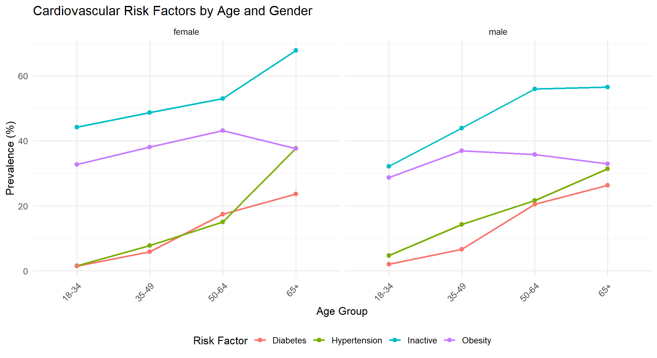
Create a comprehensive cardiovascular risk profile by demographic groups

Variables to analyze:

• Hypertension (high blood pressure)
• Obesity (BMI ≥ 30)
• Diabetes
• Physical inactivity
• Smoking

Stratify by: Age, Sex, Education

Step 1: Create Risk Indicators

cv_risk_data <- nhanes_clean %>%
  filter(Age >= 18) %>%
  mutate(
    has_hypertension = hypertension == "Yes",
    has_obesity = bmi_category == "Obese",
    has_diabetes = Diabetes == "Yes",
    inactive = PhysActive == "No",
    current_smoker = SmokeNow == "Yes",
    
    risk_count = rowSums(
      across(c(has_hypertension, has_obesity, has_diabetes,
               inactive, current_smoker), ~ as.numeric(.)),
      na.rm = TRUE
    )
  )

Step 2: Calculate Risk Prevalence

cv_risk_summary <- cv_risk_data %>%
  filter(!is.na(age_group), !is.na(Gender)) %>%
  group_by(age_group, Gender) %>%
  summarise(
    n = n(),
    hypertension_pct = mean(has_hypertension, na.rm = TRUE) * 100,
    obesity_pct = mean(has_obesity, na.rm = TRUE) * 100,
    diabetes_pct = mean(has_diabetes, na.rm = TRUE) * 100,
    inactive_pct = mean(inactive, na.rm = TRUE) * 100,
    smoking_pct = mean(current_smoker, na.rm = TRUE) * 100,
    mean_risk_count = mean(risk_count, na.rm = TRUE),
    .groups = "drop"
  ) %>%
  mutate(across(where(is.numeric), ~round(., 1)))

Step 3: Results

cv_risk_summary %>%
  arrange(age_group, Gender) %>%
  head(10)

Step 4: Visualization

cv_risk_summary %>%
  select(age_group, Gender, hypertension_pct, obesity_pct, 
         diabetes_pct, inactive_pct) %>%
  pivot_longer(
    cols = ends_with("_pct"),
    names_to = "risk_factor",
    values_to = "prevalence"
  ) %>%
  mutate(
    risk_factor = str_remove(risk_factor, "_pct"),
    risk_factor = str_to_title(risk_factor)
  ) %>%
  ggplot(aes(x = age_group, y = prevalence, 
             color = risk_factor, group = risk_factor)) +
  geom_line(linewidth = 1) +
  geom_point(size = 2) +
  facet_wrap(~Gender) +
  labs(
    title = "Cardiovascular Risk Factors by Age and Gender",
    x = "Age Group",
    y = "Prevalence (%)",
    color = "Risk Factor"
  ) +
  theme_minimal(base_size = 13) +
  theme(
    legend.position = "bottom",
    axis.text.x = element_text(angle = 45, hjust = 1)
  )

Resources & Next Steps

Key R Packages for Demographic Analysis

Data Wrangling:

• tidyverse - Complete data science toolkit
• rio - Universal data import/export
• janitor - Data cleaning helpers

Survey Analysis:

• survey - Complex survey design analysis
• srvyr - Survey data + dplyr syntax
• weights - Weighted statistics

Demographic Analysis:

• DemoTools - Demographic methods
• demography - Mortality/fertility
• popbio - Population biology

Learning Resources

Free Books:

• R for Data Science
• Advanced R
• ggplot2 book

Demographic Analysis:

• IPUMS training
• DHS Program tutorials
• WHO indicators guide

Practice:

• Tidy Tuesday
• Our World in Data
• NHANES tutorials

What We Covered Today

✅ Importing and exploring demographic/health data
✅ Data cleaning and transformation
✅ Creating demographic indicators
✅ Age-sex analysis patterns
✅ Socioeconomic gradients
✅ Data visualization
✅ Reproducible workflows
✅ Real-world applications

Next Steps in Your Learning

1. Practice with real data
   • Download DHS, MICS, or census data
   • Replicate published analyses
2. Learn visualization
   • Master ggplot2
   • Create publication-quality figures
3. Statistical analysis
   • Regression models
   • Survival analysis
   • Multilevel models
4. Advanced topics
   • Survey weights
   • Missing data methods
   • Age-standardization

Your Workshop Toolkit

Files you’ll receive:

• ✅ This slide deck (.qmd)
• ✅ Practice workbook (.Rmd)
• ✅ Sample NHANES dataset (.csv)
• ✅ Complete code scripts (.R)
• ✅ Exercise solutions
• ✅ Resource list

All materials are reproducible and yours to keep!

Thank You!

Questions?

Contact & Resources:

• Workshop materials: [GitHub repository]
• Email: [your email]
• Further learning: [Resource links]

Remember

The best way to learn R is by doing. Start with small projects, build confidence, and gradually tackle more complex analyses!

“In God we trust. All others must bring data.” - W. Edwards Deming