Libraries

1library(tidyverse)

1: Recall relevant libraries. In this post we require dplyr and ggolot2 which are available in tidyverse. For more background on it , please watch V#1 to V#4
. These videos are in Urdu/Hindi so appologies from others but codes are available to all for reproducing all the contents. Complete code is given in video link for bar graph here

Outline

bar graph: single categorical variable

Histogram : for continuous variable

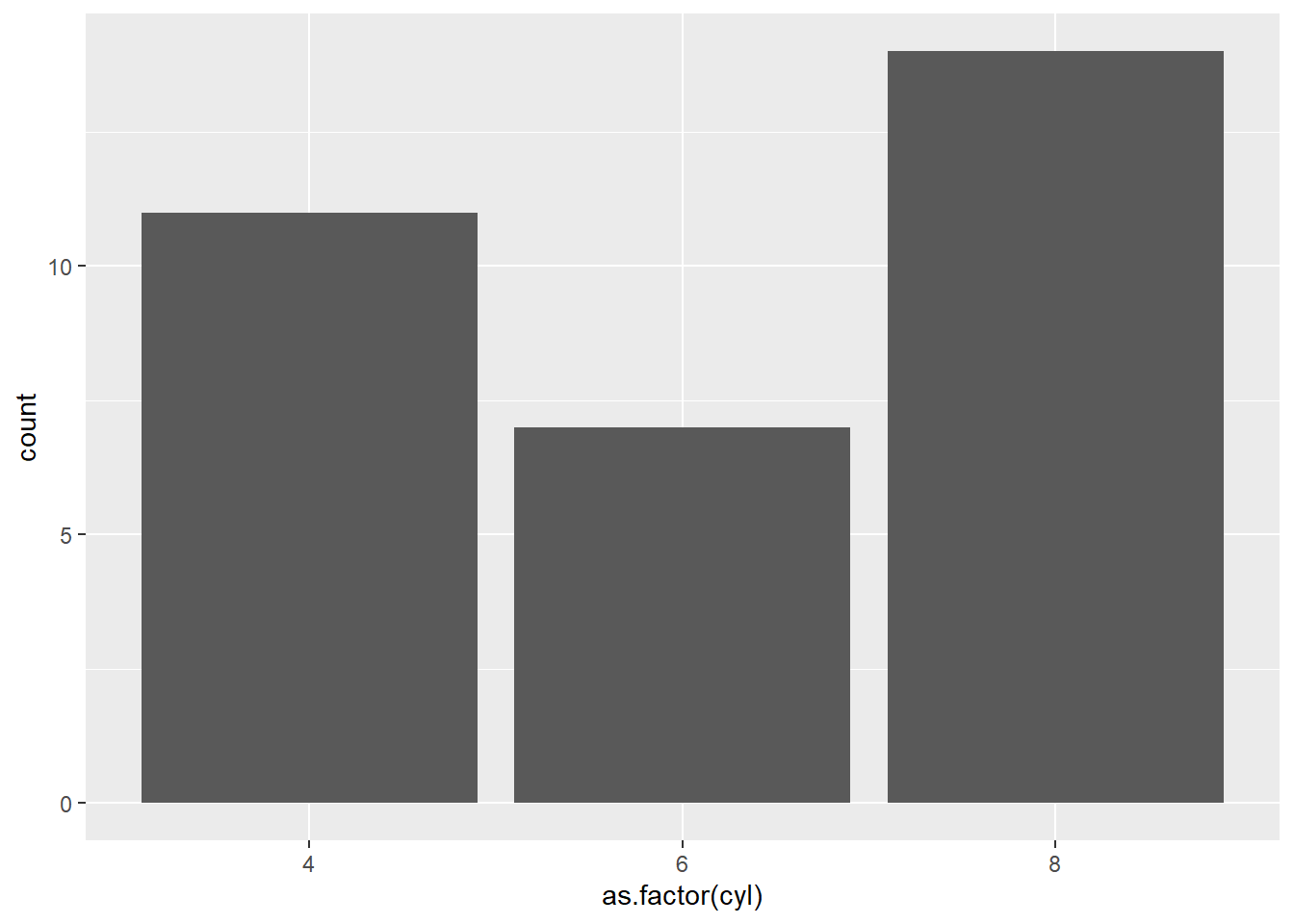
bar graph in ggplot2

1ggplot(mtcars) +
2  aes(x = as.factor(cyl)) +
3  geom_bar()

1: Read data in ggplot2
2: read data and define aesthetics
3: Mention which graph you want to make. I am using geom_bar as I have single categorical variable. If I want scatter plot, I will use geom_point()

2: uniform color. Color is for the border, fill is for the inside

ggplot(mtcars, aes(x=as.factor(cyl) )) +
  geom_bar(color="blue", fill=rgb(0.1,0.4,0.5,0.7) )

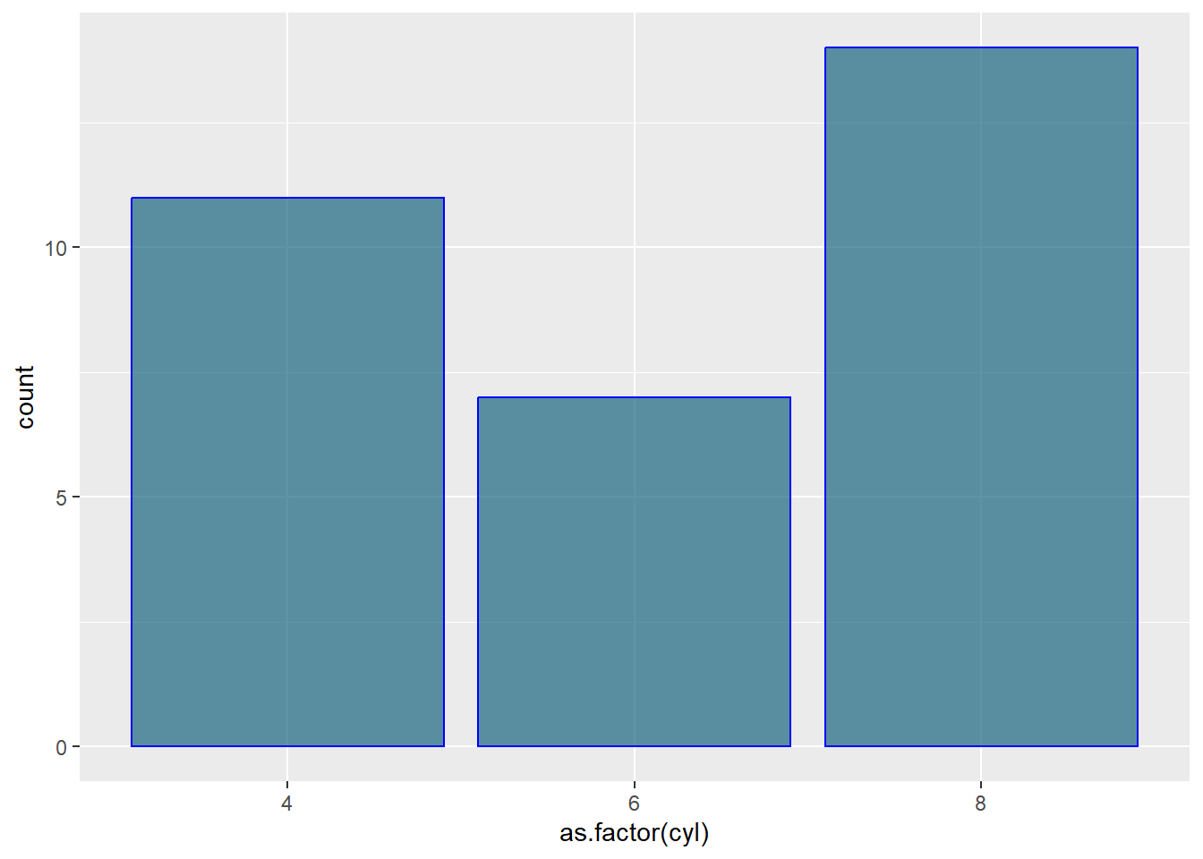
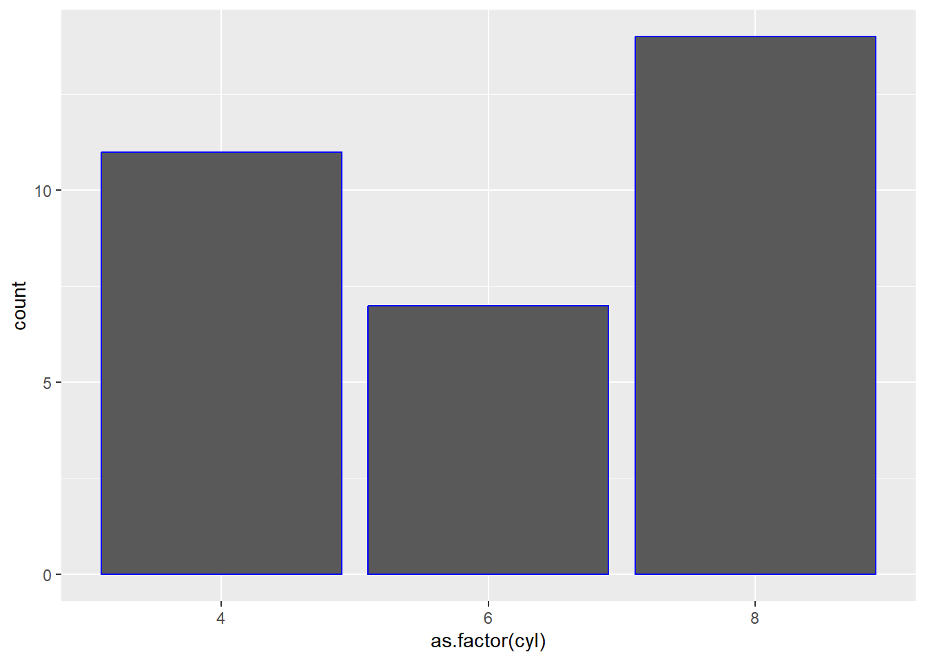
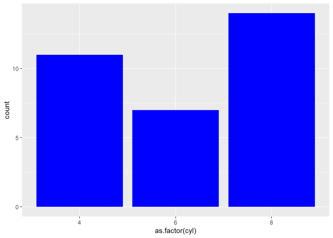
color="blue" means border of bar graph while fill means complete bar

ggplot(mtcars)+
  aes(x=as.factor(cyl))+
  geom_bar(color="blue")  # Color is the border

ggplot(mtcars)+
  aes(x=as.factor(cyl))+
  geom_bar(fill="blue")

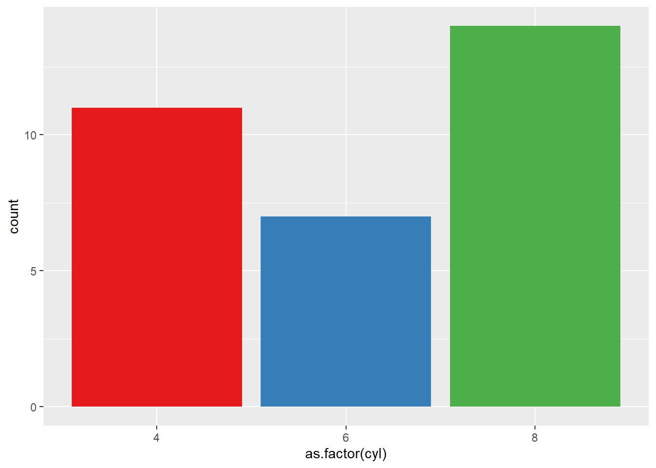
3: Using Hue

ggplot(mtcars, aes(x=as.factor(cyl), fill=as.factor(cyl) )) + 
  geom_bar( )+
  scale_fill_hue(c = 40) +
  theme(legend.position="none")

4: Using RColorBrewer

ggplot(mtcars, aes(x=as.factor(cyl), fill=as.factor(cyl) )) + 
  geom_bar( ) +
  scale_fill_brewer(palette = "Set1") +
  theme(legend.position="none")

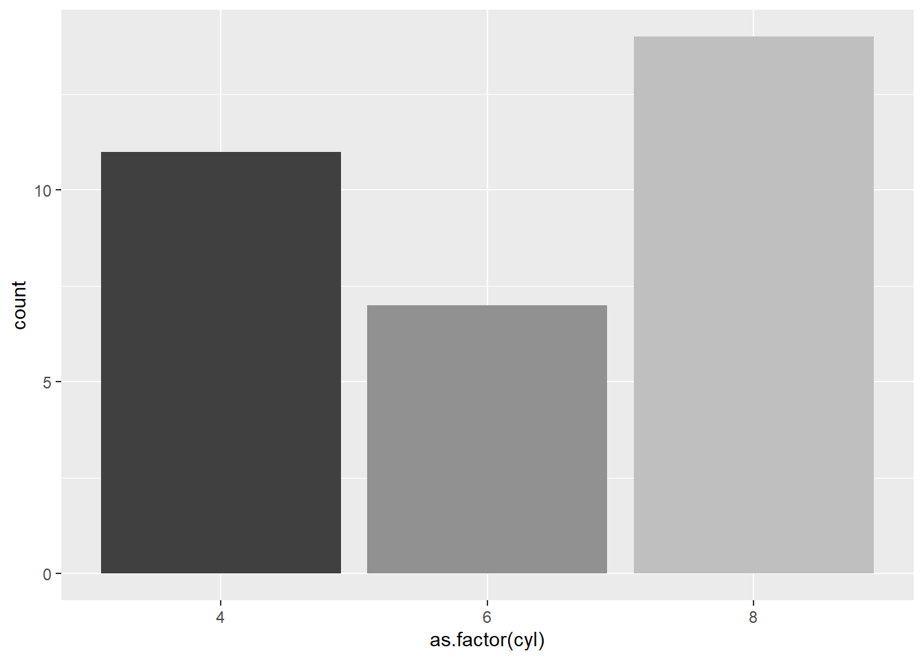
5: Using greyscale:

ggplot(mtcars, aes(x=as.factor(cyl), fill=as.factor(cyl) )) + 
  geom_bar( ) +
  scale_fill_grey(start = 0.25, end = 0.75) +
  theme(legend.position="none")

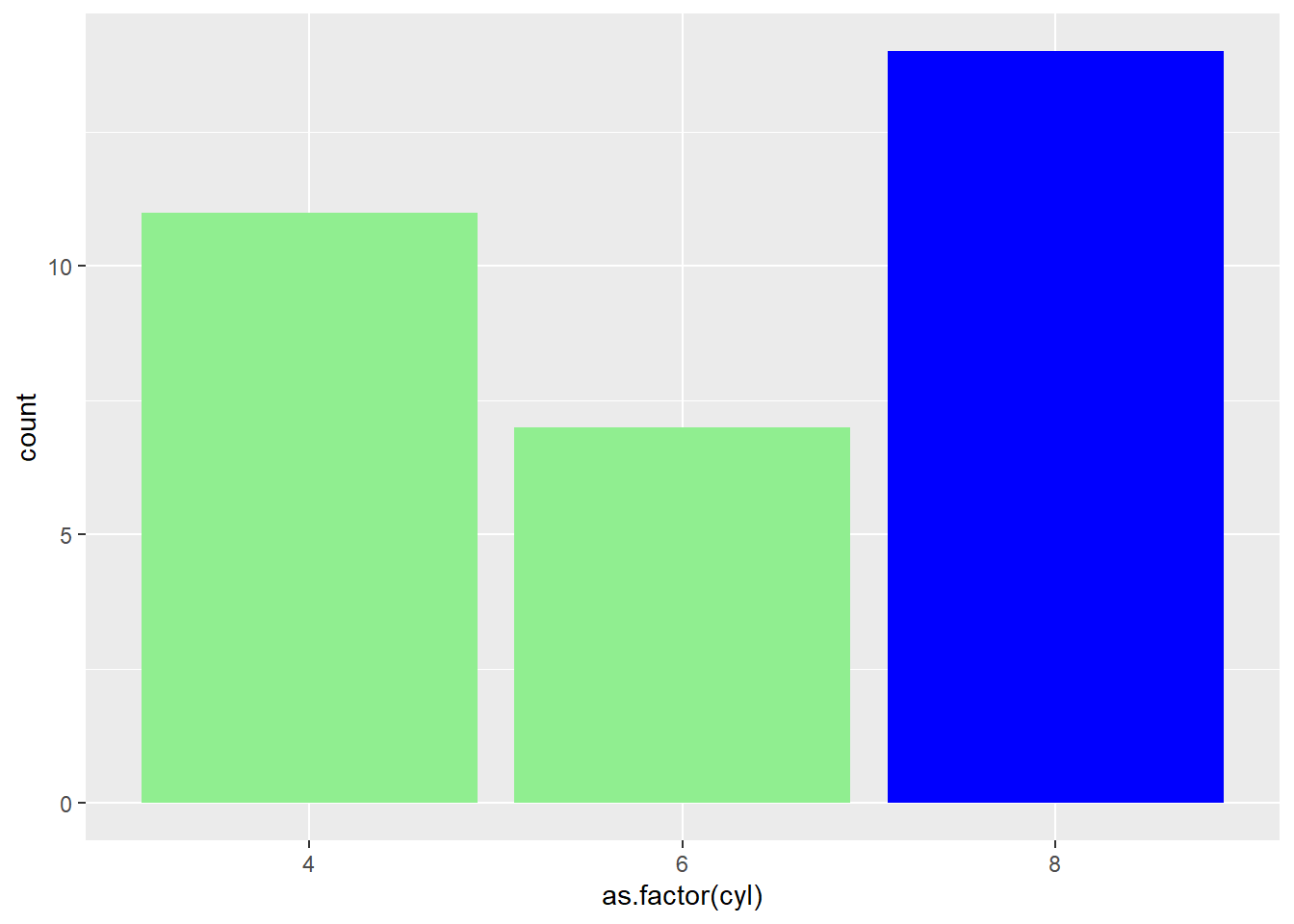
6: Set manualy

ggplot(mtcars, aes(x=as.factor(cyl), fill=as.factor(cyl) )) +  
  geom_bar( ) +
  scale_fill_manual(values = c("lightgreen", "lightgreen", "blue") ) +
  theme(legend.position="none")

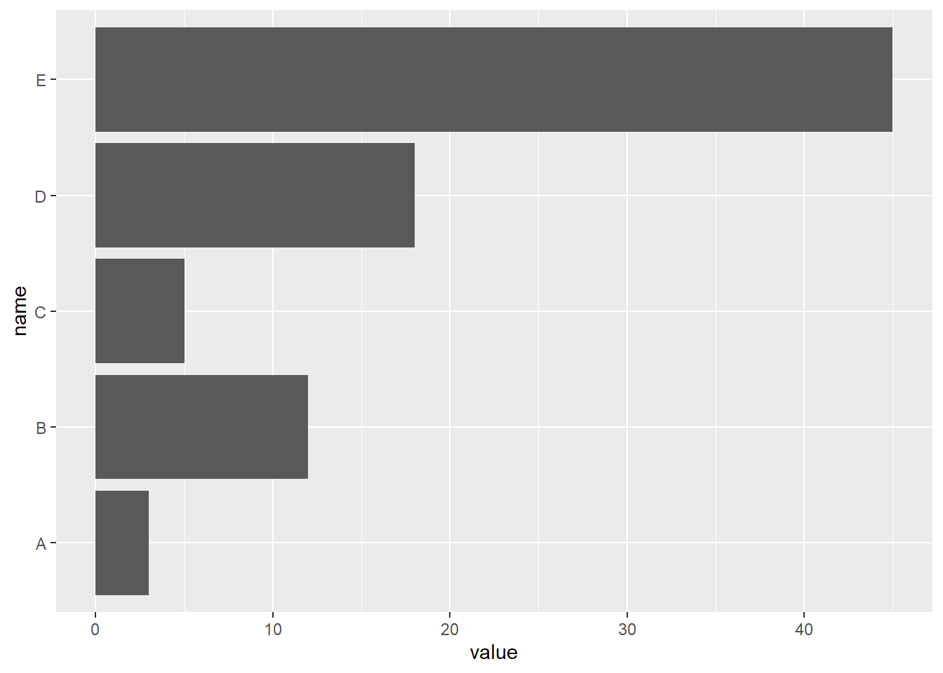
Create data

data <- data.frame(
  name=c("A","B","C","D","E") ,  
  value=c(3,12,5,18,45)
)

1ggplot(data) +
2aes(x=name, y=value) +
3  geom_bar(stat = "identity") +
  coord_flip()

1: data
2: aesthetics
3: geom_bar 4 flip coordinates

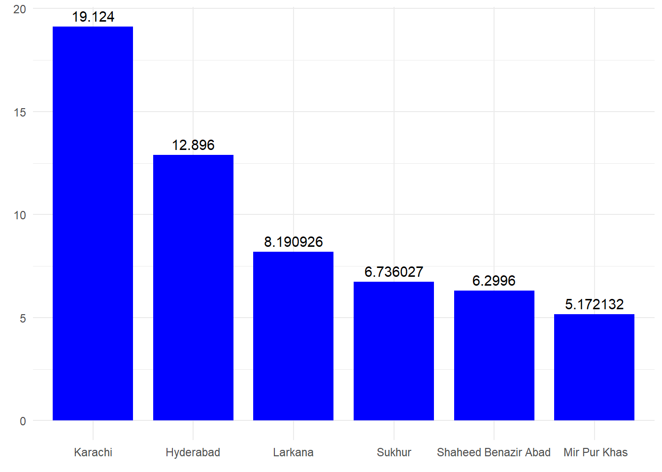
Create 2023 Census data

data <- data.frame(
  name=c("Karachi",
         "Hyderabad",
         "Larkana",
        " Mir Pur Khas",
         "Shaheed Benazir Abad",
         "Sukhur"
  ) ,  
  value=c(19124000,
          12896000,
          8190926,
          5172132,
          6299600,
          6736027
  )
)
data <- data |> mutate(population=value/1000000)

ggplot(data, aes(x=name, y=population))+ 
  geom_bar(stat = "identity", width=0.9) +
  theme_minimal()+
  geom_text(aes(label=population), vjust=-.5)

ggplot(data, aes(x=name, y=population)) + 
  geom_bar(stat = "identity", width=0.9, fill="blue") +
  theme_minimal()+
  geom_text(aes(label=population), vjust=-.5)

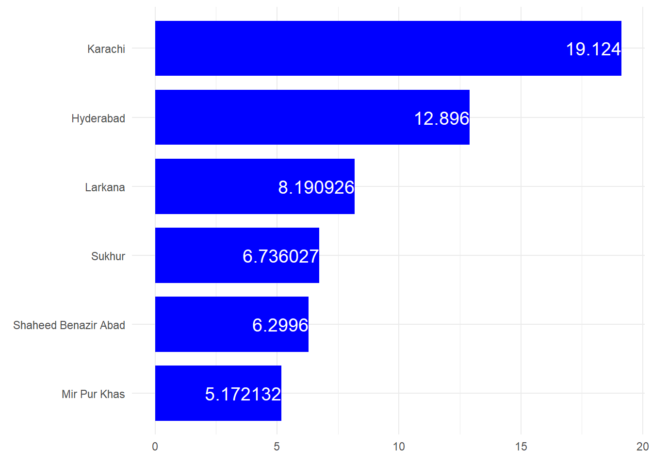
Some more modifications

  ggplot(data,aes(x=reorder(name,-population),y=population))+geom_bar(stat="identity", fill="blue", width = 0.8)+
  theme_minimal()+
  geom_text(aes(label=population), vjust=-0.5) +
  labs(x=element_blank(),
       y=element_blank())

ggplot(data,aes(x=reorder(name,population),y=population))+geom_bar(stat="identity", fill="blue", width = 0.8)+
    theme_minimal()+
    geom_text(aes(label=population), hjust=1, col="white", size=5) +
    labs(x=element_blank(),
         y=element_blank()) +coord_flip()

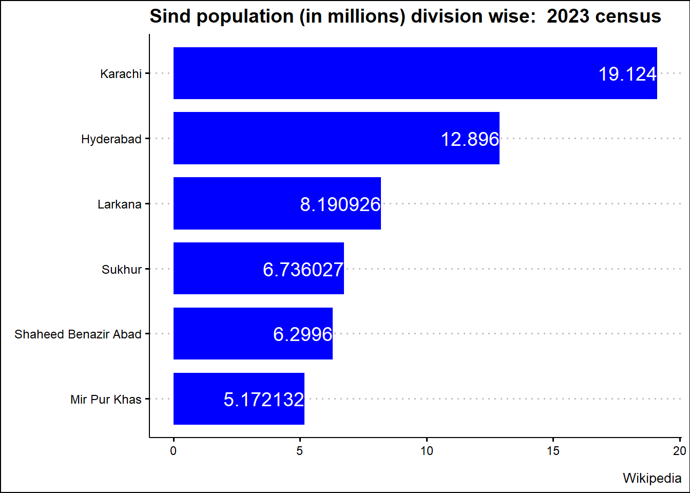
library(ggthemes)
ggplot(data, aes(x = reorder(name, population), y = population)) + geom_bar(stat =
                                                                                "identity",
                                                                              fill = "blue",
                                                                              width = 0.8) +
    theme_minimal() +
    geom_text(
      aes(label = population),
      hjust = 1,
      col = "white",
      size = 5
    ) +
    labs(x = element_blank(),
         y = element_blank()) + coord_flip() + 
    labs(title = "Sind population (in millions) division wise:  2023 census",
         caption = "Wikipedia") +
  theme_clean(
  )

This is a work by Zahid Asghar, any feedback is highly encouraged.